Download
1 / 60
740 likes | 1.19k Views
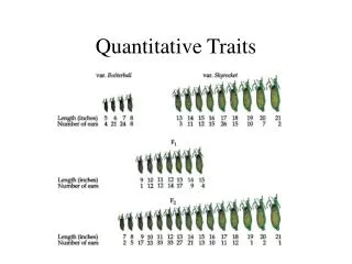
Lecture 26: Quantitative Traits VI. Date: 11/21/02 Parent-offspring finished Sib pairs Twins. Review: Parent-Offspring Regression.

E N D
Lecture 26: Quantitative Traits VI Date: 11/21/02 Parent-offspring finished Sib pairs Twins
Review: Parent-Offspring Regression • Assume (1) insubstantial epistasis, (2) equal phenotypic variation in sexes and generations, (3) no general environmental effects contributing to resemblance, and (4) no assortative mating. • When regressing offspring phenotype on parent phenotype, the regression slope is an estimate of 0.5 times the narrow-sense heritability . • When regressing offspring phenotype on the midparent phentoype, the regression slope is a direct estimate of h2.
Multiple Offspring Suppose there are n offspring in each family. The dependent variable becomes the average offspring phenotype. Making all previous assumptions, we have
Unequal Family Size • When there are unequal numbers of offspring in each family, we would like to weight each family’s contribution to the analysis in such a way as to minimize the sampling error in the heritability estimate. • The weight should naturally take into consideration the number of offspring sampled. Presumably families with more offspring “count” more (are weighted heavier).
Within/Between Family Phenotypic Variance • The among-family phenotypic variance is where Cov(S) is the phenotypic covariance of sibs and t is called the intraclass correlation. • An estimate of the within-family phenotypic variance (due to differences among individuals of the same family) is given by:
Residual Variance • The linear regression we consider is: • The residual error variance consists of • the variance attributable deviations of the “true” family means from the linear prediction (independent of sample size) • sampling variance (dependent on sample size).
Components of Residual Variance • Sampling variance is estimated by: • The variance of true offspring family means is: • Variance accounted for by linear regression: For midparent, there is factor of 0.5 on right.
Total Residual Variance • Thus, the variance of true family means from the regression is given by: • So the residual variance is the sum:
Weighted Least Squares • So the weights for families that minimize the sampling variance of the regression coefficient are: • And the weighted least-squares regression coefficient is:
Unequal Family Size – Conclusions • The weight approaches a limiting value as ni becomes large. After a while, there is little gain by sampling more offspring. • When t is large, this limit is achieved more rapidly. When there is little within family variation, you need measure only a few offspring to get a good estimate. • Since the weights are a function of the regression coefficient, it would seem impossible to perform the analysis. It’s OK, just iterate.
Relaxing Assumptions • If the mean or variance of traits differ between the sexes, then the data can be normalized (subtract mean and divide by standard deviation), such that both now have mean 0 and variance 1. • Begin analysis.
Precision of Estimates • Assume the parent and offspring phenotypes are bivariate normal. • Then the sampling distribution of the regression coefficient is normal with number of parent/offspring pairs
Precision of Estimates When midparent value is used, make the following substitutions: When multiple offspring used, make the following substitution: When unequal family sizes used, the slope estimate becomes:
Sib Analysis – Intro • Sometimes parent data is not available • Can’t identify the parent • Parent no longer alive • Three types of analysis • full sib • half sib • full and half sib • Assume random sample of families and random mating of parents.
Half-Sib • If epistatic effects are small and common environmental effects do not contribute to resemblance of sibs, then 4 times the covariance of half sibs is an estimate of additive genetic variance and approximately twice the parent-offspring covariance.
Half-Sib – Common Environment • A shared environment is the biggest potential problem with half-sib analysis. • One solution is to use paternal half-sibs that are raised by multiple mothers. • A common design is one sib from each mother. • The analysis is ANOVA-based. Regression causes problems because of non-independence between pairs of sibs.
Half-Sib – ANOVA • The linear model used is: • The residual error (eij) is caused by: • environmental variance • genetic variance among mothers • segregation in father • dominance • Assume eij are uncorrelated and have common variance (within family variance)
Half-Sib – Sire Effects • The si are called sire effects and are assumed to have mean 0 (true when fathers are random sample). • Let the variance among sire effects be • Critical ANOVA assumption is that the random effects are uncorrelated. So, we must assume • Also note that the phenotypic covariance between members of a group equals the variance among groups.
Half-Sib Covariation When epistatic effects are minimal:
General Approach • Specify the linear model. • State assumptions of model and write an expression for the total phenotypic variance in terms of the components. • Write the components of variance associated with the model in terms of the covariance between classes of relatives. • Using the resemblance between relatives results, write these covariances between relatives as sums of causal components of variance (e.g. additive, dominance, epistatic, etc).
Method of Moments Estimators of Variance Components Plug in sample estimates:
Heritability Estimator intraclass correlation unimportant for N>20
Hypothesis Testing • Estimates of variance components are unbiased regardless of the distribution of the linear effects (no normality assumption require). • Hypothesis tests assume normal distribution and constant variance. • Normality of observed data does not guarantee linear effects are normally distributed.
Testing Heritability>0 • Assuming normality and constant variance. • A significant result implies:
Meaning of Significant Result • A lack of significance could merely mean that there was insufficient power. • Standard errors can provide more information by indicating the accuracy of the estimates. • To calculate standard errors we need the sampling variances of the observed mean squares.
Sampling Variance of Variance Components Assume equal family size. Standard errors obtained by substituting MSE and taking square roots. These are LARGE SAMPLE estimators.
Sampling Variance of Heritability - t is the intraclass correlation. - Obtained by delta method. Again, a large sample estimator.
Confidence Intervals • Assume normally distributed effects and homogenous variance. • Often, researchers simply assume parameter estimates are approximately normally distributed. Then standard errors are used to calculate confidence intervals +/- 1.96*standard error.
Confidence Interval – Among Family Variance Assume equal size sibships. MSs/MSe
Confidence Interval - Heritability Assume equal size sibships.
Example • The wild parsnip cannot self-fertilize. Assume that all its seeds produced by one plant are therefore half-sibs. Two flowers are unlikely to be pollinated with pollen from the same plant when there is lots of pollen from multiple sources floating around. • Select 20 random plants. • Collect 10 seeds from each and plant. • Analyze the mature plants.
Example – Data • Some plants died prior to assay. • 5 plants had 10 offspring assayed. • 8 plants had 9 offspring assayed. • 4 plants had 8 offspring assayed • 1 plant each had 7, 6, and 4 offspring assayed. • UNBALANCED DESIGN
Example - Calculations • MSe = 0.0370 • MSs = 0.1156 • Var(s) = 0.0092 • Var(e) = 0.0370 • Var(z) = 0.0462 • t = Var(s)/Var(z) = 0.20 • h2 = 4t = 0.80 (no epistatic effects) • SE(h2) = 4SE(t) = 0.32 • F = 3.12 with 19 and 151 degrees of freedom => p-value < 0.01.
Example - Analysis • Maternal half-sibs used. • It is actually quite conceivable that many of the seeds were full sibs. • Both of these possibilities affect heritability estimates in the same way. Increase or decrease?
Resampling Procedures • Since the hypothesis tests assume normality and equal variance and since many of the results were contingent on a large sample, numerical procedures that do not make these assumptions have been employed. • jacknife: delete one family from dataset at a time and recalculate estimates. • bootstrap: draws samples of same size with replacement from dataset. • permutation: randomize the half-sibs among families which generates null distribution under assumption
Full-Sib • Twice the inraclass correlation gives an estimate of heritability if dominance, environmental, and epistatic effects are minimal. These are BIG assumptions for full sibs, so full sibs are not often used to estimate heritibility. • Combined with half-sib analysis, full sib analysis can provide information on the relative role of dominance and environmental effects.
Half-Sib/Full-Sib Design • Mate each of N randomly selected fathers with several different females and sample multiple offspring from each female. • The offspring of one female are full sibs. • The offspring of different females with same father are half-sibs.
Linear Model i is the ith sire j is the jth “dam” mated to the ith sire k is the kth offspring of the ith sire and jth dam
Derivation • We now convert observable components of variance to covariance between relatives. • The residual variance is the variance within full-sib families: Covariance between full sibs = variance between families
Total Variance common environment special environment
Estimation • Thus, four times the sire component provides and estimates of the additive genetic variance. • The difference between the dam component and the sire component provides an estimate of the impact of the dam and common environment. The latter two cannot be separated.
Sample Size Specifics T is total number of individuals in experiment. M is the mean number of dams per sire. niis the total number of offspring for the ith sire.
Hypothesis Testing • Assume normality and balanced design. • A test for significant sire effects: • A test for significant dam effects:
Unbalanced Hypothesis Testing where Q = c1MS1 + c2MS2 + ...+cmMSm
Interpretation • Since variance of sires is an estimate of genetic additive effect, a significant sire effect indicates significant additive effect.
Twins • Monozygotic twins are genetically identical (MZ). • Dizygotic twins are full sibs (DZ). • A greater amount of phenotypic variability is assumed between DZ vs. MZ twins when genetics underly the trait.
Twins – Linear Model • We define a simple linear model for both types of twins (MZ and DZ): • eij is a result of segregation (in DZ) and environmental variance (in both DZ and MZ). • Assume DZ and MZ twin pairs are a random sample such that E(bi) = 0.