Download
1 / 18
270 likes | 650 Views
Low Density Parity Check codes. Performance similar to turbo codes Do not require long interleaver to achieve good performance Better block error performance Error floor occurs at lower BER Decoding is not trellis based Iterative decoding More iterations than turbo decoding

E N D
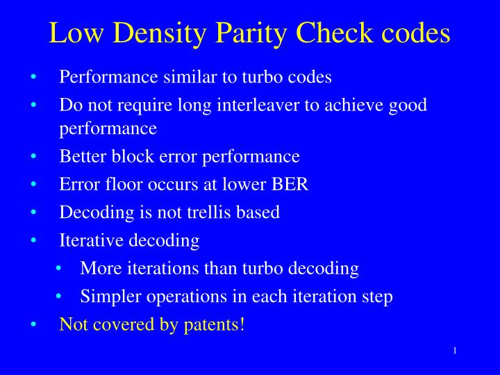
Low Density Parity Check codes • Performance similar to turbo codes • Do not require long interleaver to achieve good performance • Better block error performance • Error floor occurs at lower BER • Decoding is not trellis based • Iterative decoding • More iterations than turbo decoding • Simpler operations in each iteration step • Not covered by patents!
Introduction • A binary parity check matrix Hn-kn • C = { vGF(2)n : vHT = 0 } • (Regular) LDPC code: The null space of a matrix H which has the following properties: • Its J rows are not necessarily linearly independent • 1s in each row • 1s in each column • No pair of columns has more than one common 1 • and are small compared to the number of rows (J) and columns (n) in H • Density r = /n = /J • Irregular: The number of 1s in rows/columns may vary
Example • J = n = 15 • = = 4
Gallager’s LDPC codes • Select and • Form a kk matrix H consisting of submatrices H1,...,H, each of dimensions kk • H1 is a matrix such that its ith row has its 1s confined to columns (i-1)+1 to i. • The other submatrices are column permutations of H1 • The actual column permutations define the properties of the code
Gallager’s LDPC codes: Example • Select = 4, = 3 • Column permutations for H2 and H3 selected so that no two columns have more than one 1 in common • (20,7,6) code
Rows and parity checks • Each row of H forms a parity check • Let Al be the set of rows {h1(l),...,h(l)} that have a one in position l, i. e. the set of parity checks on symbol l. • Since no pair of columns has more than one common 1, any code bit other than bit l is checked by at most one of the rows in Al. • Thus there are rows orthogonal on l, and any error pattern of weight /2 can be decoded by one-step majority logic decoding. However, (especially when is small) this gives poor performance • Gallager proposed two iterative decoding algorithms, one hard decision based and one soft decision based
Brief overview of graph theoretic notations • An undirected graph G(V,E) • Degree of a vertex/node : Number of edges adjacent to it • Adjacent edges: Connected to the same vertex • Path in a graph: Alternating sequence of vertices and edges (starting and ending in a vertex), where all vertices are distinct except for maybe the first and the last • A tree: A graph without cycles • Connected graph: There is a path between any pair of vertices • Bipartite graph: the set of vertices can be partitioned into two disjoint parts; so that each edge goes from a vertex in one part to a vertex in the other
Graphical description of LDPC codes • Tanner graph: A bipartite graph G(V,E), where • V = V1 V2 • V1is a set of ncode-bit nodes v0,...,vn-1, each representing one of the n code bits • V2is a set of Jcheck nodes s0,...,sJ-1, each representing one of the J parity checks • There is an edge between v V1and s V2iff the code-bit corresponding to v is contained in the parity check s. • No cycles of length 4 for the Tanner graph of an LDPC code
Decoding of LDPC codes • Several decoding techniques available. Listed in order of increasing complexity (and improving performance): • Majority logic decoding (MLG) • Bit flipping (BF) • Weighted bit flipping (WBF) • Iterative decoding based on belief propagation (IDBP) also known as the sum-product algorithm (SPA) • A posteriori probability decoding (APP)
Decoding notation • Codeword = channel input : v = (v0,..., vn-1), binary • Assume BPSK modulation on AWGN channel • Channel output : y = (y0,..., yn-1) • Hard decisions : z = (z0,..., zn-1), zj = 1 (0)yj > (<) 0 • Rows of H : h1,..., hJ • Syndrome : s = (s1,..., sJ) = z HT, sj = z hj = l=0...n-1zlhj,l • Parity failure : at least one syndrome bit nonzero • Error pattern e = v + z • Syndrome : s = (s1,..., sJ) = e HT, sj = e hj = l=0...n-1elhj,l
Majority logic decoding • One-step MLG (see Chapter 8*) • Let Al be the set of rows {h1(l),...,h(l)} that have a one in position l, i. e. the set of parity checks on symbol l. • Set of parity checks orthogonal on code bit l: • Sl = { s= z h = e h = l=0...n-1elhl : h Al } • If a majority of the parity checks on bit l are satisfied; conclude that el = 0. Otherwise, assume that el = 1. • This decoding is guaranteed to result in a correct decoding if at most /2 errors occur. • Problem: is by assumption a small number.
Bit flipping decoding • Introduced by Gallager in 1961 • Hard decision decoding: First, form the hard decisions z = (z0,..., zn-1) • Compute the parity check sumss = (s1,..., sJ) = z HT, sj = z hj = l=0...n-1zlhj,l • For each bit l, find fl = the number of failed parity checks for bit l • Let S = the set of bits for which fl is large • Flip the value of the bits in S • Repeat from a) until all parity checks are satisfied, or a maximum number of iterations have been reached
Bit flipping decoding (continued) • Let S = the set of bits for which fl is large • For example: • S = the set of bits for which fl exceeds some threshold that depends on the code parameters: , , minimum distance and channel SNR. If decoding fails, try again with reduced value of • Simple alternative: S = the set of bits for which fl is maximum • Comments: • If few errors occur, decoding should commence in a few iterations • On a poor channel, the number of iterations should be (allowed to grow) large • Improvement: Adaptive thresholds
Weighted MLG and BF decoding • Use weighting to include soft decision/reliability information in the decoding decision • Hard decision decoding: First, form the hard decisions z = (z0,..., zn-1) • Weight: | yj|(l)min = min{| yi| : 0in-1, hj,i =1, h Al } • The reliability of the jth parity check on l • Weighted MLG: Hard decision on • El = s Sl (2s-1)| yj|(l)min • ...where Sl = { s= z h = e h = l=0...n-1elhl : h Al } • Weighted BF: • Compute the parity checks s = (s1,..., sJ) = z HT • For each bit l, compute El . • Flip the value of the bit for which El is largest • Repeat from a) until all parity checks are satisfied, or a maximum number of iterations have been reached
The sum-product decoding algorithm • Iterative decoding based on belief propagation • Symbol-by-symbol SISO: The goal is to compute • P( vl | y ) • L(vl) = log ( P( vl = 1| y )/P( vl = 0| y ) ) • A priori values: plx = P( vl = x), x{0,1} • qj,lx,(i) = P(vl = x |check sums Al \ {hj} at ith iteration} • hj = (hj,0, hj,1, ..., hj,n-1); support of hj = B(hj) = { l : hj,l = 1} • j,lx,(i) = P(sj=0| vl = x,{vt:tB(hj)\{l}}) tB(hj)\{l}qj,tvt,(i) • qj,lx,(i+1) = j,l(i+1) ht Al \ {hj}t,lx,(i) • j,l(i+1) chosen so that qj,l0,(i+1) +qj,l1,(i+1) =1 • P (i)(vl = x | y )=l(i) hj Alj,lx,(i-1) • l(i) chosen so that P (i)(vl = 0| y )+ P (i)(vl = 1 | y )=1
The SPA on the Tanner graph qj,lx,(i) qj,mx,(i) qj,nx,(i) qj,lx,(i+1) j,lx,(i) a,lx,(i) b,lx,(i) qj,mx,(i+1) qj,nx,(i+1) vl sj + • qj,lx,(i) = P(vl = x |check sums Al \ {hj} at ith iteration} • j,lx,(i) = P(sj=0| vl = x,{vt:tB(hj)\{l}}) tB(hj)\{l}qj,tvt,(i) • qj,lx,(i+1) = j,l(i+1) ht Al \ {hj}t,lx,(i)
Suggested exercises • 17.1-17.11