Inverse Laplace Transformations

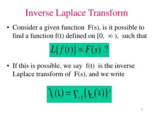
1. Inverse Laplace Transformations Dr. Holbert February 27, 2008 EEE 202

2. Inverse Laplace Transform • Consider that F(s) is a ratio of polynomial expressions • The n roots of the denominator, D(s) are called the poles • Poles really determine the response and stability of the system • The m roots of the numerator, N(s), are called the zeros EEE 202

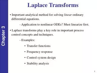
3. Inverse Laplace Transform • We will use partial fractions expansion with the method of residues to determine the inverse Laplace transform • Three possible cases (need proper rational, i.e., n>m) • simple poles (real and unequal) • simple complex roots (conjugate pair) • repeated roots of same value EEE 202

4. 1. Simple Poles • Simple poles are placed in a partial fractions expansion • The constants, Ki, can be found from (use method of residues) • Finally, tabulated Laplace transform pairs are used to invert expression, but this is a nice form since the solution is EEE 202

5. 2. Complex Conjugate Poles • Complex poles result in a Laplace transform of the form • The K1 can be found using the same method as for simple poles WARNING: the "positive" pole of the form –+j MUST be the one that is used • The corresponding time domain function is EEE 202

6. 3. Repeated Poles • When F(s) has a pole of multiplicity r, then F(s) is written as • Where the time domain function is then • That is, we obtain the usual exponential but multiplied by t's EEE 202

7. 3. Repeated Poles (cont’d.) • The K1j terms are evaluated from • This actually simplifies nicely until you reach s³ terms, that is for a double root (s+p1)² • Thus K12 is found just like for simple roots • Note this reverse order of solving for the K values EEE 202

8. The “Finger” Method • Let’s suppose we want to find the inverse Laplace transform of • We’ll use the “finger” method which is an easy way of visualizing the method of residues for the case of simple roots (non-repeated) • We note immediately that the poles are s1 = 0 ; s2 = –2 ; s3 = –3 EEE 202

9. The Finger Method (cont’d) • For each pole (root), we will write down the function F(s) and put our finger over the term that caused that particular root, and then substitute that pole (root) value into every other occurrence of ‘s’ in F(s); let’s start with s1=0 • This result gives us the constant coefficient for the inverse transform of that pole; here: e–0·t EEE 202

10. The Finger Method (cont’d) • Let’s ‘finger’ the 2nd and 3rd poles (s2 & s3) • They have inverses of e–2·t and e–3·t • The final answer is then EEE 202

11. Initial Value Theorem • The initial value theorem states • Oftentimes we must use L'Hopital's Rule: • If g(x)/h(x) has the indeterminate form 0/0 or /  at x=c, then EEE 202

12. Final Value Theorem • The final value theorem states • The initial and final value theorems are useful for determining initial and steady-state conditions, respectively, for transient circuit solutions when we don’t need the entire time domain answer and we don’t want to perform the inverse Laplace transform EEE 202

13. Initial and Final Value Theorems • The initial and final value theorems also provide quick ways to somewhat check our answers • Example: the ‘finger’ method solution gave • Substituting t=0 and t=∞ yields EEE 202

14. Initial and Final Value Theorems • What would initial and final value theorems find? • First, try the initial value theorem (L'Hopital's too) • Next, employ final value theorem • This gives us confidence with our earlier answer EEE 202

15. Solving Differential Equations • Laplace transform approach automatically includes initial conditions in the solution • Example: For zero initial conditions, solve EEE 202

16. Class Examples • Find inverse Laplace transforms of • Drill Problems P5-3, P5-5 (if time permits) EEE 202