Download
1 / 40
430 likes | 600 Views
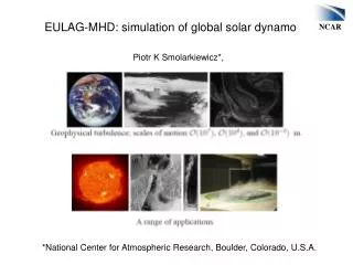
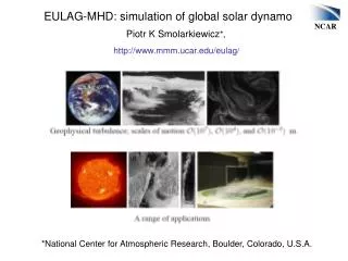
The Solar Dynamo. Peter A. Gilman High Altitude Observatory National Center for Atmospheric Research SHINE 2002 Summer Workshop. Layers of the Sun. Solar Cycle Model “Tracks”. Where Next? Longitudinal Wave Number m > 0 ( non axisymmetric models ) Predictions of Subsequent Cycles.

E N D
The Solar Dynamo Peter A. Gilman High Altitude Observatory National Center for Atmospheric Research SHINE 2002 Summer Workshop High Altitude Observatory (HAO) – National Center for Atmospheric Research (NCAR) The National Center for Atmospheric Research (NCAR) is operated by the University Corporation for Atmospheric Research (UCAR) under sponsorship of the National Science Foundation. An Equal Opportunity/Affirmative Action Employer.
Solar Cycle Model “Tracks” • Where Next? • Longitudinal Wave Number m > 0(non axisymmetric models) • Predictions of Subsequent Cycles
What is a Hydromagnetic Dynamo? A conducting fluid in which the flow maintains the magnetic field “permanently” against ohmic dissipation. • Some General Requirements: • Dynamos must be 3D in space. “Cowling’s theorem” precludes 2D dynamos (proved 1934) • Irony: Most solar dynamos ARE 2D; circumvents Cowling’s theorem by parametric representation of 3D induction processes • Simple estimates of ohmic decay time for, say, a star, are not enough to determine whether will have dynamo action (primordial fields are sometimes proposed) • Why? Because turbulence can greatly enhance dissipation. • Magnetic Reynolds number Rm must be sufficiently large
Properties that Promote Dynamo Action (inferred from observation, verified by theory) • Rotation • Convection (energy conversion) • Size (hard to make an MHD dynamo in the lab - Rm’s too small) • Complexity of flow pattern (Cowlings theorem). A particularly interesting flow property is its • KINETIC HELICITY • Is large when flow has spiral structure • Would cause lifting & twisting of initially straight field line in highly conducting fluid. • Combination of rotation and convection can lead to a lot of kinetic helicity, but can get it by other means also
Magnitude of Solar Dynamo Problem • Dominant historical strategy: • Stick to kinematic problem – specify velocities and solve for magnetic fields • Keep problem global, parameterize all smaller scale effects Advantage:Avoids all of scale problems listed above Disadvantage:Need to know how to parameterize, and how to specify velocity fields
Observational Constraints on Solar Dynamo Theory • Differential rotation with latitude, depth, time • Meridional circulation with latitude, depth, time • Convection zone depth • Existence of solar tachocline • Other motions from helioseismic interferences (synoptic maps) Structure & Velocities • Butterfly diagram for spots • Hales polarity laws • Field reversals • Phase relation in cycle between toroidal & poloidal fields • Field symmetry about equator • Field “handedness” (current helicity, magnetic helicity) • Solar cycle envelope • Cycle period – cycle amplitude relation • Active longitudes • Sunspot group tilts (Joy’s Law), asymmetries between leaders & followers • Others??? Magnetic Properties
Physical Processes That May Be Important in the Solar Dynamo Inclusion in dynamo models:Explicitly-E; Parameterized-P; Absent-N
Tracer Rotation (Reprinted from Beck, John G., A Comparison of Different Rotation Measurements , Solar Physics, 191: 47-70, 1999.)
Spectroscopic Rotation (Reprinted from Beck, John G., A Comparison of Different Rotation Measurements , Solar Physics, 191: 47-70, 1999.)
Differential Rotation from Helioseismic Analysis (Used with permission from Paul Charbonneau)
Angular Velocity Domains in Solar Convection Zone and Interior, from Helioseismology
Meridional Circulation from Helioseismology (Courtesy of JILA, University of Colorado)
Observed and Inferred Characteristics of Meridional Circulation(from a variety of sources) • Usually poleward flow in each hemisphere ~20m/sec. • Surface variations with the time 50-100%.(how much real, how much noise?) • One circulation cell replaced by two at times. • North & South hemispheres can look quite different. • Cell in one hemisphere can extend several degrees latitude to the other. • Surface Doppler & helioseismic results often do not agree. Spots as tracers show much smaller drift. • Flow amplitude likely determined by small differences among large forces (Coriolis, pressure gradients, turbulent stresses, and buoyancy?), so significant fluctuations likely. • Most mass transport well below photosphere, because flow speed observed to change slowly with depth. • Must be return flow near bottom of convection zone, but not observed yet. • Return flow amplitude should respond quickly (sound travel time?) to poleward flow changes above (has implications for cycle prediction).
Mean Field Dynamo Equations(Steenbeck, Krause, Radler, et al.) Turbulent diffusion Molecular diffusion Differential rotation and/or meridional circulation ~ Kinetic helicity of lifting and twisting (“α-effect”) on sphere, solve for axisymmetric magnetic field “Poloidal” Field “Toroidal” Field
Axisymmetric Dynamo Evolution Velocity Constraints Magnetic Constraints
Some Major Effects of Observational Constraints on Dynamo Models • Differential rotation with radius contradicted assumption in 1970s mean field models; led to putting dynamo at base of convection zone. Also contradicted 3D global convection models. • Sunspots only in low latitudes led to requirements of ~100 kG fields at base as source, because magnetic buoyancy must overcome Coriolis forces. • Tachocline differential rotation allows induction of strong toroidal fields at location where they can be held in storage until erupt as active regions. • Observed meridional circulation strong enough to determine dynamo period (correctly), over-powering combination of radial differential rotation and -effect. Peter A. Gilman
First Solar Dynamo Paradox • Mean field dynamo theory applied to sun required rotation increase inward • Global convection models predicted rotation approximately constant or cylinders, but with equatorial acceleration ~30% In 1970s prevailing view was that global convection theory must be wrong (I never shared that view). In 1980s helioseismic inferences proved both were wrong, but dynamo theory more wrong than convection theory. Conclusion Move dynamo to base of convection zone
Alternative flux tube trajectories, determined by strength of rotation, magnetic field, turbulent drag. Rotation Axis Source Toroidal Field Equator Trajectory Parallel to the Rotation Axis Trajectory Radial Schematic of Range of Trajectories of Rising Tubes Limiting Cases: Choudhuri and Gilman, 1987, ApJ., 316, 788.
Second Solar Dynamo Paradox • To produce sunspots in low latitudes requires toroidal fields ~105 gauss at the base of the convection zone (influence of Coriolis forces on rising tubes) • 105 gauss fields very hard to store – must be below convectively unstable layer (overshoot layer subadiabatic?) • 105 gauss fields are 102 x equipartition – won’t that suppress dynamo action? (but apparently does not in geo case!) Resolution Interface Dynamos Flux Transport Dynamos
Interface Dynamos(Introduced by Parker ApJ. 408, 707, 1993) Elements: Interface at base of convection zone (at tachocline) Below interface: helicity or small turbulent diffusivity small radial differential rotation large Above interface: helicity or small turbulent diffusivity large radial differential rotation small Weak diffusion across interface crucial. Solutions work: Below interface: Toroidal field largePoloidal field small Above interface: Toroidal field smallPoloidal field large
FLUX-TRANSPORT DYNAMO + MERIDIONAL CIRCULATION Pole .6R 1R .7R Equator (Dikpati & Choudhuri, 1994, A&A, 291, 975.) (Choudhuri, Schüssler, & Dikpati, 1995, A&A, 303, L29.) (Durney, 1995, SolP, 160, 213.)
Flux Transport Mean Field Dynamos Solved Including: • Meridional circulation (single celled, with surface flow toward poles) • Nonlinear and nonlocal -effect arising from twist acquired by rising buoyant flux tubes acted upon by Coriolis forces • -effect from global HD/MHD instabilities in tachocline Successes: • Reversal frequency determined by amplitude of meridional circulation • Observed meridional circulation leads to observed solar cycle period! (Relatively independent of magnitude, profile) • -effect near bottom from global HD/MHD instability in tachocline leads to correct magnetic field symmetry about equator(Hales Law)
Evolution of Magnetic FieldsIn Flux-Transport Dynamos(Dikpati Model)
How Much Solar Rotation, Meridional Circulation Theory is Needed to do Solar Dynamos?
What Would Happen Now if we did Full MHD Dynamo Simulations with the Best Available Global Convection Model? • Would still get wrong butterfly diagram (migration towards poles rather than equator) • Toroidal fields probably much too weak, diffuse • Would not be able to handle both storage of flux at the bottom, as well as bulk convection zone dynamics. • Fields too diffuse, partly because of resolution limits. Means flow in model cannot “get around” magnetic flux the way it can in real sun. • Answer may be to have hybrid dynamo, with full MHD in tachocline, but kinematic in convection zone above.
Hybrid Nonaxisymmetric Dynamo With Some MHD Properties: • 2D or 3D global MHD in the tachocline • Flux transport model for bulk convection zone, with assumed DR and MC from observations • DR from convection zone imposed on tachocline • Global m0 patterns generated in tachocline diffuse into convection zone
Hybrid Nonaxisymmetric Dynamo With Some MHD Advantages: • Avoids use of global theory of convection and differential rotation and meridional circulation that we know from previous calculations will give dynamo results in conflict with solar observations, i.e., wrong butterfly diagram • Can extend flux transport dynamos to physics-based modeling of m0 magnetic patterns • Can directly assess the relative roles played by meridional circulation and tachocline dynamics in determining dynamo properties
Power Spectrum of the Magnetic Field Power in lowest longitudinal wave numbers, integrated over all latitudes, of the observed photospheric radial magnetic field (from Kitt Peak magnetograms), averaged over Carrington rotations 1601-1611. • The segmented curve T represents the total power in each wave number • The curve S represents power in that part of the field which is symmetric about the equatorial plane • The curve A the antisymmetric part • T is simply the sum of S and A. (Reprinted from Coronal Holes and High Speed Wind Streams, edited by J. B. Zirker, c. VIII, p. 340,1977.)
Global, Quasi 2D MHD of the Solar Tachocline • MHD analog to classical GFD problems of barotropic & baroclinic instability • Magnetic field can make unstable differential rotations that are stable without it • If allow some variation in radial direction, instability can generate kinetic helicity. • Subject of continuing long term study by: Gilman, Fox, Dikpati, Cally, Miesch (in order of first involvement)
Global Quasi-2D MHD Instability of Tachocline Results(Gilman, Fox, Dikpati, Cally) • DR and TF generally unstable to global waves, particularly longitudinal wave number m = 1, sometimes also m = 2 or higher. • efolding Growth Times: few months – few years. • Longitudinal Propagation Speeds: between minimum and maximum rotation rates ( max for strong fields) • Nonlinear growth leads to “tipping” of toroidal field rings (can be same or opposite in NH and SH) • Allowing even weak radial motions leads to unstable modes with kinetic helicity -effect • Global disturbances in tachocline could set “template” for surface magnetic features.
Tipped Toroidal Ring in Longitude-latitude Coordinates Linear Solutions with Two Possible Symmetries (Cally, Dikpati, & Gilman, 2002 ApJ, submitted)
Nonlinear Evolution of Tip of Toroidal Rings Due to 2D MHD Instability Latitudeof band 60º 40º 20º Time (Cally, Dikpati, & Gilman, 2002, ApJ, submitted)
Rotation 1866-67 Source Data from Feb 17, 1993 to Apr 13, 1993 CARRINGTON LONGITUDE Rotation 1867-68 Source Data from Mar 16, 1993 to May 10, 1993 CARRINGTON LONGITUDE Rotation 1866-68 Source Data from Feb 17, 1993 to May 10, 1993 CARRINGTON LONGITUDE Synoptic Flow from Magnetic Patterns P. Ambrož from Solar Physics, 199: 251-266, 2001.
Possible Causes of Dominance of (1) Dipole Symmetry & (2) N-S Asymmetries (1) Location of kinetic helicity or “-effect” (top versus bottom)Others? (2) Asymmetries in differential rotation and/or meridional circulation (3) Stochastic fluctuations
What Should AffectCycle Strength? • Differential rotation amplitude (doesn’t vary much) • Meridional circulation amplitude (varies a lot) • Storage time for toroidal magnetic fields below convection zone (in tachocline) • Threshhold for magnetic flux injection into convection zone • Stochastic variations • Others?
What Should Affect Polar Field Reversals? • Random walk rate (variations unknown) • Meridional circulation (variability large fraction of mean value) • Meridional transport by nonaxisymmetricmotions (not studied yet) • In-situ magnetic flux emergence (hard to estimate) • In-situ magnetic flux submergence (also hard to estimate)
Sources of Departures from Equatorial Symmetry • Random fluctuations in flux eruption • N/S asymmetries in meridional circulation • N/S asymmetries in differential rotation • N/S asymmetries in other synoptic-scale motions A Case-Study Thought Experiment Meridional circulation was weaker, or reversed, in NH in years leading up to cycle 23 reversal, so might expect reversal later there. But in fact it was apparently earlier or the same • Possible reasons: • NH less eruption of new flux? • NH cycle phase already ahead of SH? • NH polar flux weaker to start with?