Download
1 / 33
340 likes | 371 Views
Learn about causal models, representing interventions, determining independence, and using graphs to predict effects and update beliefs efficiently.

E N D
Causal models • Recall from yesterday: • Represent relevance using graphs • Causal relevance ⇒ DAGs • Quantitative component = joint probability distribution • And so clear definitions for independence & association • Connect DAG & jpd with two assumptions: • Markov: No edge ⇒ Independent given direct parents • Faithfulness: Conditional independence ⇒ No edge
Three uses of causal models • Represent (and predict the effects of) interventions on variables • Causal models only, of course • Efficiently determine independencies • I.e., which variables are informationally relevant for which other ones? • Use those independencies to rapidly update beliefs in light of evidence
Representing interventions • Central intuition: When we intervene, we control the state of the target variable • And so the direct causes of the target variable no longer matter • But the target still has its usual effects • Directly applying current to the light bulb ⇒ light switch doesn’t matter, but the plant still grows
Representing interventions • Formal implementation: • Add a variable representing the intervention, and make it a direct cause of the target • When the intervention is “active,” remove all other edges into the target • Leave intact all edges directed out of the target, even when the intervention is “active”
Light Switch Plant Growth Light Bulb Representing interventions • Example:
Light Switch Plant Growth Current Light Bulb Representing interventions • Example: • Add a manipulation variable as a “cause”
Light Switch Plant Growth Current Light Bulb Representing interventions • Example: • Add a manipulation variable as a “cause” that does not matter when it is inactive Inactive Inactive Manipulation
Light Switch Plant Growth Current Light Bulb Light Switch Plant Growth Current Light Bulb Representing interventions • Example: • Add a manipulation variable as a “cause” that does not matter when it is inactive • When it is active, Inactive Inactive Manipulation Active Manipulation
Light Switch Plant Growth Current Light Bulb Light Switch Plant Growth Current Light Bulb Representing interventions • Example: • Add a manipulation variable as a “cause” that does not matter when it is inactive • When it is active, break the incoming edges, but leave the outgoing edges Inactive Inactive Manipulation Active Manipulation
Representing interventions • Straightforward extension to more interesting types of interventions • Interventions away from current state • Multi-variate interventions • Etc. • Key: For all of these, the “intervention operator” takes a causal graphical model as input, and yields a causal graphical model as output • “Post-intervention CGM” is an ordinary CGM
Why randomize? • Standard scientific practice: randomize Treatment to find its Effects • E.g., don’t let people decide on their own whether to take the drug or placebo • What is the value of randomization? • Randomization is an intervention • ⇒ All edges into T will be broken, including from any common causes of T and E! • ⇒ If T E, then we must have: T → E
Treatment Effect Why randomize? • Graphically, ?
Treatment UnobservedFactors Effect Why randomize? • Graphically, ?
Treatment UnobservedFactors Effect Why randomize? • Graphically, ?
Treatment UnobservedFactors Effect Why randomize? • Graphically, ?
Treatment UnobservedFactors Effect Why randomize? • Graphically, ?
Three uses of causal models • Represent (and predict the effects of) interventions on variables • Causal models only, of course • Efficiently determine independencies • I.e., which variables are informationally relevant for which other ones? • Use those independencies to rapidly update beliefs in light of evidence
Determining independence • Markov & Faithfulness ⇒ DAG structure determines all statistical independencies and associations • Graphical criterion: d-separation • X and Y are independent given S iffX and Y are d-separated given S iffX and Y are not d-connected given S • Intuition: X and Y are d-connected iff information can “flow” from X to Y along some path
d-separation • C is a collider on a path iff A→ C ← B • Formally: • A path between A and B is active given S iff • Every non-collider on the path is not in S; and • Every collider on the path is either in S, or else one of its descendants is in S • X and Y are d-connected by S iff there is an active path between X and Y given S
d-separation • Surprising feature being exploited here: • Conditioning on a common effect induces an association between independent causes • Motivating example: Gas Tank → Car Starts ← Spark Plugs • Gas and Plugs are independent, but if we know that the car doesn’t start, then they’re associated • In that case, learning Gas = Full changes the likelihood that Plugs = Bad • And similarly if Car Starts→Emits Exhaust
d-separation • Algorithm to determine d-separation: • Write down every path between X and Y • Edge direction is irrelevant for this step • Just write down every sequence of edges that lies between X and Y • But don’t use a node twice in the same path
d-separation • Algorithm to determine d-separation: • Write down every path between X and Y • For each path, determine whether it is active by checking the status of each node on the path • The node is not active if either: • N is a collider + not in S (and no descendants of N are in S); or • N is not a collider and in S. • I.e., “multiply” the “not”s to get the node status • Any node not active ⇒ path not active
d-separation • Algorithm to determine d-separation: • Write down every path between X and Y • For each path, determine whether it is active by checking the status of each node on the path • Any path active ⇒ d-connected ⇒ X & Y associated No path active ⇒ d-separated ⇒ X & Y independent
Exercise FoodEaten Weight Metabolism d-separation • Exercise and Weight given Metabolism? • E→ M → W • Blocked! M isan included non-collider • E→ FE → W • Unblocked! FE isa non-included non-collider • ⇒ EW | M
Exercise FoodEaten Weight Metabolism d-separation • Metabolism and FE given Exercise? • M→ W ← FE • Blocked! W isa non-included collider • M← E → FE • Blocked! E isan included non-collider • ⇒ M FE | E
Exercise FoodEaten Weight Metabolism d-separation • Metabolism and FE given Weight? • M→ W ← FE • Unblocked! W isan included collider • M← E → FE • Unblocked! E isa non-included non-collider • ⇒ MFE | W
Updating beliefs • For both statistical and causal models, efficient computation of independencies ⇒ efficient prediction from observations • Specific instance of belief updating • Typically, “just” compute conditional probabilities • Significantly easier if we have (conditional) independencies, since we can ignore variables
Bayes (and Bayesianism) • Bayes’ Theorem: • proof is trivial… • Interpretation is the interesting part: • Let D be the observation and T be our target variable(s) of interest • ⇒ Bayes’ theorem says how to update our beliefs about T given some observation(s)
Bayes (and Bayesianism) Likelihoodfunction • Terminology: Priordistribution Posteriordistribution Data distribution
Bayes and independence • Knowing independencies can greatly speed Bayesian updating • P(C | E, F, G) = [complex mess] • Suppose C independent of F, G given E • ⇒ P(C | E, F, G) = P(C | E) = [something simpler]
Exercise FoodEaten Weight Metabolism Updating beliefs • Compute: P(M = Hi | E = Hi, FE = Lo) • FE M | E⇒P(M | E, FE) = P(M | E) • And P(M | E) is a term in theMarkov factorization!
Looking ahead… • Have: • Basic formal representation for causation • Fundamental causal asymmetry (of intervention) • Inference & reasoning methods • Need: • Search & causal discovery methods