Download
1 / 29
290 likes | 410 Views
A tutorial on Sites : An analytical toolbox for ecoregional conservation planning. Sandy Andelman, Ian Ball, Frank Davis, David Stoms University of California, Santa Barbara December, 1999. Tutorial Outline.

E N D
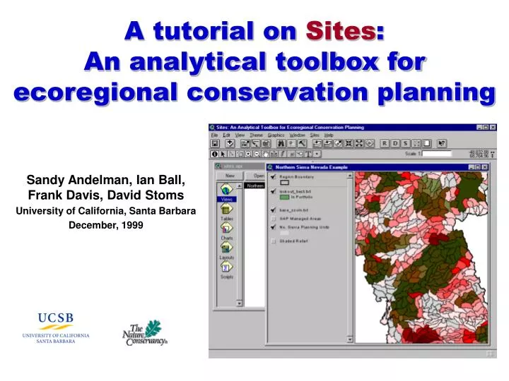
A tutorial on Sites: An analytical toolbox for ecoregional conservation planning Sandy Andelman, Ian Ball, Frank Davis, David Stoms University of California, Santa Barbara December, 1999
Tutorial Outline This slideshow is designed as a tutorial on the features of the toolbox. The remainder of the slideshow is organized into two parts: • the features of the toolbox: • the portfolio (or sites) selection module • the graphical interface that links the module to the GIS database • examples of the features in operation with different goals, costs, and assumptions
The planning problem The Nature Conservancy (TNC) recently initiated a new program to assemble ecoregional portfolios of conservation lands that collectively represent viable examples of all native species and plant communities. The initial steps involve selecting a set of target elements (i.e., species and communities), identifying levels of representation for each target, and then identifying a set of sites (the “conservation portfolio”) from among a larger set of “planning units” within the ecoregion. This portfolio provides a systematic basis for site planning and acquisition. The overall objective of the portfolio selection process is to minimize the “cost” of the portfolio while ensuring that all conservation goals for representation and spatial configuration have been met.
TNC Requirements • Given the large number of elements and sites, it is virtually impossible without the aid of computer automation for conservation planners to evaluate all possible alternative portfolios. • From TNC's perspective, the major limitations of current tools fall into three general categories: too technical, insufficient documentation and/or inadequate testing, or overly simplistic decision rules. • TNC contracted with UCSB to develop a prototype spatial decision support system for selecting planning units to accommodate TNC's portfolio design methodology. We call the system ‘Sites’.
Site Selection Module Within Sites, the portfolio selection software is called the Site Selection Module (SSM). It was originally written by Ian Ball and Hugh Possingham of the University of Adelaide in Australia as a stand-alone Windows-based program. SSM: • provides 2 heuristic procedures--simulated annealing and “greedy” • allows the analyst to control the spatial configuration of the conservation portfolio • facilitates exploration of alternative goals and assumptions • allows planning units to be required or excluded in a portfolio • compares the portfolio to the distribution of a given conservation element
Objective Function SSM attempts to minimize the total cost of a portfolio: Or in plain language, Total Portfolio Cost = (cost of selected sites) + (penalty cost for not meeting the stated conservation goals for each element) + (cost of spatial dispersion of the selected sites as measured by the total boundary length of the portfolio).
Simulated Annealing Simulated Annealing evaluates complete alternative portfolio at each step, and compares a very large number of alternative portfolios to identify a good solution. The procedure begins with a random set, and then at each iteration swaps planning units in and out of that set and measures the change in cost. If the change tends to improve the set, the new set is carried forward to the next iteration until the maximum number of iterations is reached. This algorithm is slower than the Greedy heuristic but tends to find better solutions.
Greedy Heuristic The Greedy Heuristic is a stepwise, iterative procedure. At each step, it scans each planning unit that is not yet in the portfolio and selects the one that reduces the total cost by the greatest amount, until all element goals have been satisfied to the extent possible. At this point according to the objective function it is not ‘cost effective’ to add any more planning units. This procedure, which has been widely used in previous studies, has the advantage of being extremely fast and producing reasonably efficient solutions.
Spatial Complexity Spatial complexity can be included in SSM in any of 3 ways. • Contiguity: For a conservation portfolio of a given size, the shorter the total boundary length around selected planning units, the more compact will be the portfolio. One objective of the SSM, therefore, is to minimize the total length of the boundary of the portfolio. • Minimum Area: It is not enough that the portfolio itself be contiguous and compact but the areas for some species must be adequately large. In SSM, the minimum area that is considered adequate for a sub-population or sub-region can be specified. • Separation Distance: It may also be important to ensure that occurrences of some elements are sufficiently separated to mitigate the effects of localized catastrophes. If a separation distance is specified, then the program will favor solutions where there are at least 3 planning units that are separated by that minimum distance.
Planning Units Sites is best suited (but not restricted) to the situation where an ecoregion has been divided into a set of candidate sites, called “planning units” that completely fill the region and are of roughly the same size and shape. Examples include regular grids, watersheds, landscapes, or any other geographic features that make sense from data compilation and conservation planning perspectives. These are the basic building blocks for assembling a portfolio. Therefore the delineation of planning units should be made carefully. There are several different files that are used to characterize the planning units.
Input Files Files for planning units • name.dat (contains a unique identifying number for each unit) • puvspr.dat (area of each element in each planning unit) • bound.dat (optional, contains length, or cost, of each boundary between planning units--default is that all boundaries are equal) • cost.dat (optional, contains the fixed “cost” of selecting a planning unit--default is that all costs are equal) • pustat.dat (optional, contains status of planning units, e.g., locked in or out of portfolio--default is that all units are available) • puxy.dat (optional, contains coordinates of each planning unit--required if separation rule is invoked) Files for elements • species.dat (for each element, contains number/name, representation goal, penalty factor and spatial goals)
SSM Outputs There are six possible types of output files based on the five choices under 'Save Options' in the Input Editor window.
The ArcView Interface A customized ArcView (.apr) project is the graphical user interface to the toolbox. It includes a ‘Sites’ menu and a series of new buttons for running three parts of the SSM--InEdit, Site Selection, and Distribution Preparer--and for displaying solutions.
Input Editor The Input Editor is run from the ‘Sites’menu or from the ‘I’ button. It is where the analyst selects the algorithm, the cost threshold and boundary modifier values, and the output files to be saved. The directories for input and output are also set in this dialog form. You must click the ‘Save’ button to set these choices.
Running Site Selection The site selection module is run by clicking on the ‘Run Site Selection’ menu or the ‘S’ button. SSM will then be executed with your current values from the Input Editor. A window will appear that shows current status and summary information and will tell you when it is finished.
Displaying a Solution After SSM has selected an alternative portfolio, you can display the selected planning units. First, make the base map of planning units the active theme by clicking on it in the Table of Contents. Click on the ‘Display Reserve’ menu, which will open a dialog box asking you for the field with the ID numbers. Select the appropriate field and ‘OK’. Choose the appropriate scenario file in your output folder, and a new map will be displayed in the View window.
Displaying a “Summed” Solution Planners may not want just a good alternative but also to see how robust the solution is. To do this, select the 'Sum Runs' option under 'Save Options’ in the Input Editor. This will generate a file (ending in ssoln.txt) that lists the number of times each planning unit was selected out of the total number of annealing runs. (Not available for Greedy solutions). This file can be displayed by selecting ‘Display Summed Solution’ in the ‘Sites’ menu. The rest of the procedure is the same as displaying a single solution. The results are displayed as a color gradient from gray (never selected) to dark red (most frequently selected).
Displaying a Species Distribution It can be helpful to see the distribution of planning units in a portfolio in relation to the individual biodiversity elements being represented. First select the 'Run Distribution Preparer' to create a data file. Then use ‘Display Species Distribution’ in the ‘Sites’ menu (or click the 'D' button). Identify the element to be displayed by name or code number, and it will be drawn as a red crosshatch.
Displaying Planning Unit Status The status file shows which planning units are locked into a portfolio and which are locked out. With a theme selected, click on the ‘S’ button or chose ‘Display status’ from the ‘Sites’ menu. The status will be displayed. The number of categories might include status 0 or 1 (planning units neither locked in nor out of the reserve), status 2 (planning units locked in), and status 3 (planning units locked out). Not all of these categories may be present.
Changing Planning Unit Status Select a number of planning units whose status you wish to change using the usual ArcView selection tool. After you have selected the planning units (highlighted in yellow), go to the 'Sites' menu and choose 'Change Status of Selected Planning Units'. The program prompts whether the status of these planning units is to be cleared, locked in or locked out of the system. Select tool
Show Contents of a Planning Unit Planners often want to see what biodiversity elements are in a planning unit to understand why it was selected for an alternative portfolio. Select a planning unit(s) in the solution theme and the 'Show Contents' menu item. The listing contains the element code, element name, and area of the selected planning unit that the planning unit contributed towards meeting the representation goals. Select tool
Chart of Targets Met Site selection algorithms will never meet all representation goals exactly. To show how many types are under- and over-represented in a given solution, the toolbox creates a histogram of the proportions of the representation goals (1.0 being perfectly met) for all elements. In the Tables View, Open or Add a targets-met table whose name will look something like file_mvbest.txt. Click on the ‘Chart Targets Met Data’ item in the ‘Sites’ menu to get a pre-formatted histogram.
Effect of the algorithm Effect of boundary modifier (clustering of portfolio) Effect of changing costs Effect of changing representation goals Effect of locking in units in the portfolio Examples for the Northern Sierra Nevada Ecoregion
Effect of the Algorithm SSM provides 2 algorithms for selecting portfolios. Annealing is slower but tends to find more efficient solutions, while the Greedy heuristic is faster but less efficient. This slide shows the difference between solutions by the 2 algorithms. Simulated annealing is in green; greedy in red (boundary modifier = 0.2 in both cases). Greedy does less well at clustering because it can not drop an isolated planning unit once it has been selected.
Effect of Boundary Modifier Because it is desirable for nature reserves to be both compact and contiguous, one objective of the annealing algorithm is to minimize the total length of the boundary of the portfolio. This slide shows how increasing the boundary modifier (BM) in the InEdit window affects the clustering in the solution. BM = 0.0 BM = 0.2 BM = 1.0
Effect of Changing Costs In these examples, we show how the assumptions about costs affect the solution. In each figure, the green planning units are from the original solution (BM = 0.2), which set Cost = Area + Suitability. Red shows the solution if Cost = Area only (left), if Cost = 0 (center, all planning units cost the same), and when a cost threshold of 1 million is assigned (right). The threshold is similar to a budget constraint, except that not all costs are in economic units. Cost = Area Cost = 0 Cost threshold = 1M
Effect of Changing Representation Goals In this example, we show how the goals for representing each vegetation community can be modified and the how that affects the solution. The green planning units are the base alternative (BM = 0.2) with the original representation goals, while the units in red crosshatch satisfy the goals reduced by half. This is done by substituting a new species.dat file.
Effect of Locking Units in the Portfolio Defining the starting reserve system is an important consideration in designing a portfolio and generally you will want to consider several alternatives. For example, you may consider an alternative that starts by fixing existing national parks and other formally designated reserves. Green shows the original solution again, while red shows an alternative where existing nature reserves (small inset map) are forced in.
Highlights • Sites responds to the need for portfolio selection to be as efficient or cost-effective as possible, given the competing social and economic demands for land and water. It also addresses the concern that portfolio design should be repeatable, so that it can be readily re-evaluated and modified over time as conditions change and new information is acquired. • Sites assists planners in sorting through a large volume of data to identify good initial solutions to this complex, multi-objective problem. • The planning team must still review the initial solutions and modify them using local knowledge, judgment, and other evidence not considered in the planning approach.