Download

1 / 42
420 likes | 673 Views
One-Factor Experiments. Andy Wang CIS 5930-03 Computer Systems Performance Analysis. Characteristics of One-Factor Experiments. Useful if there’s only one important categorical factor with more than two interesting alternatives Methods reduce to 2 1 factorial designs if only two choices

E N D
One-Factor Experiments Andy Wang CIS 5930-03 Computer Systems Performance Analysis
Characteristics ofOne-Factor Experiments • Useful if there’s only one important categorical factor with more than two interesting alternatives • Methods reduce to 21 factorial designs if only two choices • If single variable isn’t categorical, should use regression instead • Method allows multiple replications
Comparing Truly Comparable Options • Evaluating single workload on multiple machines • Trying different options for single component • Applying single suite of programs to different compilers
When to Avoid It • Incomparable “factors” • E.g., measuring vastly different workloads on single system • Numerical factors • Won’t predict any untested levels • Regression usually better choice • Related entries across level • Use two-factor design instead
An Example One-Factor Experiment • Choosing authentication server for single-sized messages • Four different servers are available • Performance measured by response time • Lower is better
The One-Factor Model • yij = j + eij • yij is ith response with factor set at level j • is mean response • j is effect of alternative j • eij is error term
One-Factor Experiments With Replications • Initially, assume r replications at each alternative of factor • Assuming a alternatives, we have a total of ar observations • Model is thus
Sample Datafor Our Example • Four alternatives, with four replications each (measured in seconds) A B C D 0.96 0.75 1.01 0.93 1.05 1.22 0.89 1.02 0.82 1.13 0.94 1.06 0.94 0.98 1.38 1.21
Computing Effects • Need to figure out and j • We have various yij’s • Errors should add to zero: • Similarly, effects should add to zero:
Calculating • By definition, sum of errors and sum of effects are both zero, • And thus, is equal to grand mean of all responses
Calculating j • j is vector of responses • One for each alternative of the factor • To find vector, find column means • Separate mean for each j • Can calculate directly from observations
Calculating Column Mean • We know that yij is defined to be • So,
Calculating Parameters • Sum of errors for any given row is zero, so • So we can solve for j:
Parametersfor Our Example Server A B C D Col. Mean .9425 1.02 1.055 1.055 Subtract from column means to get parameters Parameters -.076 .002 .037 .037
EstimatingExperimental Errors • Estimated response is • But we measured actual responses • Multiple ones per alternative • So we can estimate amount of error in estimated response • Use methods similar to those used in other types of experiment designs
Sum of Squared Errors • SSE estimates variance of the errors: • We can calculate SSE directly from model and observations • Also can find indirectly from its relationship to other error terms
SSE for Our Example • Calculated directly: SSE = (.96-(1.018-.076))^2 + (1.05 - (1.018-.076))^2 + . . . + (.75-(1.018+.002))^2 + (1.22 - (1.018 + .002))^2 + . . . + (.93 -(1.018+.037))^2 = .3425
Allocating Variation • To allocate variation for model, start by squaring both sides of model equation • Cross-product terms add up to zero
Variation In Sum of Squares Terms • SSY = SS0 + SSA + SSE • Gives another way to calculate SSE
Sum of Squares Termsfor Our Example • SSY = 16.9615 • SS0 = 16.58256 • SSA = .03377 • So SSE must equal 16.9615-16.58256-.03377 • I.e., 0.3425 • Matches our earlier SSE calculation
Assigning Variation • SST is total variation • SST = SSY - SS0 = SSA + SSE • Part of total variation comes from model • Part comes from experimental errors • A good model explains a lot of variation
Assigning Variationin Our Example • SST = SSY - SS0 = 0.376244 • SSA = .03377 • SSE = .3425 • Percentage of variation explained by server choice
Analysis of Variance • Percentage of variation explained can be large or small • Regardless of which, may or may not be statistically significant • To determine significance, use ANOVA procedure • Assumes normally distributed errors
Running ANOVA • Easiest to set up tabular method • Like method used in regression models • Only slight differences • Basically, determine ratio of Mean Squared of A (parameters) to Mean Squared Errors • Then check against F-table value for number of degrees of freedom
ANOVA Table forOne-Factor Experiments Compo- Sum of % of Degrees of Mean F- F- nent Squares Var. Freedom Square Comp Table yar 1 SST=SSY-SS0 100 ar-1 Aa-1 F[1-; a-1,a(r-1)] e SSE=SST-SSA a(r-1)
ANOVA Procedurefor Our Example Compo- Sum of % of Degrees of Mean F- F- nent Squares Variation Freedom Square Comp Table y 16.96 16 16.58 1 .376 100 15 A .034 8.97 3 .011 .394 2.61 e .342 91.0 12 .028
Interpretationof Sample ANOVA • Done at 90% level • F-computed is .394 • Table entry at 90% level with n=3 and m=12 is 2.61 • Thus, servers are not significantly different
One-Factor Experiment Assumptions • Analysis of one-factor experiments makes the usual assumptions: • Effects of factors are additive • Errors are additive • Errors are independent of factor alternatives • Errors are normally distributed • Errors have same variance at all alternatives • How do we tell if these are correct?
Visual Diagnostic Tests • Similar to those done before • Residuals vs. predicted response • Normal quantile-quantile plot • Residuals vs. experiment number
What Does The Plot Tell Us? • Analysis assumed size of errors was unrelated to factor alternatives • Plot tells us something entirely different • Very different spread of residuals for different factors • Thus, one-factor analysis is not appropriate for this data • Compare individual alternatives instead • Use pairwise confidence intervals
Could We Have Figured This Out Sooner? • Yes! • Look at original data • Look at calculated parameters • Model says C & D are identical • Even cursory examination of data suggests otherwise
Looking Back at the Data A B C D 0.96 0.75 1.01 0.93 1.05 1.22 0.89 1.02 0.82 1.13 0.94 1.06 0.94 0.98 1.38 1.21 Parameters -.076 .002 .037 .037
What Does This PlotTell Us? • Overall, errors are normally distributed • If we only did quantile-quantile plot, we’d think everything was fine • The lesson - test ALL assumptions, not just one or two
One-Factor Confidence Intervals • Estimated parameters are random variables • Thus, can compute confidence intervals • Basic method is same as for confidence intervals on 2kr design effects • Find standard deviation of parameters • Use that to calculate confidence intervals • Typo in book, pg 336, example 20.6, in formula for calculating j • Also typo on pg. 335: degrees of freedom is a(r-1), not r(a-1)
Confidence Intervals For Example Parameters • se = .169 • Standard deviation of = .042 • Standard deviation of j = .073 • 95% confidence interval for = (.932, 1.10) • 95% CI for = (-.225, .074) • 95% CI for = (-.148,.151) • 95% CI for = (-.113,.186) • 95% CI for = (-.113,.186)
Unequal Sample Sizes in One-Factor Experiments • Don’t really need identical replications for all alternatives • Only slight extra difficulty • See book example for full details
Changes To HandleUnequal Sample Sizes • Model is the same • Effects are weighted by number of replications for that alternative: • Slightly different formulas for degrees of freedom