Download
1 / 33
330 likes | 332 Views
= ?. +. Unstable mode. Unstable mode. NL. Grid States and Nonlinear Selection in Parametrically Excited Surface Waves. Tamir Epstein and Jay Fineberg The Racah Institute of Physics The Hebrew University of Jerusalem. Stable mode. Grid State – Spatial mode locking

E N D
= ? + Unstable mode Unstable mode NL Grid States and Nonlinear Selection in Parametrically Excited Surface Waves Tamir Epstein and Jay Fineberg The Racah Institute of Physics The Hebrew University of Jerusalem Stable mode Grid State – Spatial mode locking new family of Superlattice structures
Talk outline: • Motivation – why study parametrically excited waves • (especially with a lot of excitation frequencies) • Linear stability and the 2 frequency phase diagram • What exactly is a Grid State? • Control of the system using a 3rd frequency • Grid states in nonlinear optics…
Well -studied nonlinear systems: Patterns: Single excited spatial mode + secondary instabilities e.g. R-B, Couette-Taylor, Faraday Instability... Chaos: Order - Disorder in the temporal domain Turbulence: A large number of concurrently excited modes • Motivation: • What structures are selected when a few distinctly different nonlinear modes • are allowed to interact? • Selection criteria / interaction mechanisms? • Routes to complexity in both space and time
Localized States Superlattice states H. Arbell and J.F. PRL 81, 4384 (1998) H. Arbell and J.F. PRL 84, 654 (2000) ) H. Arbell and J.F.PRL. 85, 756-60 (2000)
Propagating dissipative solitons – single frequency drivingwith high dissipation O. Lioubashevski, H. Arbell, and J. F., PRL 76, 3959 (1996 ). O. Lioubashevski and J. F., Phys. Rev. E63, 5302 (2001).
CCD Imaging system CCD Gradient lit cylinder 12 lamps 1.2 meter Gradient lit cylinder Temp. control Shaker Reflecting surface wave PC Experimental System
l ½w w/2 ↔ k a>ac Squares The Faraday Instability: Single Frequency Forcing:a(w) = a·cos(wt) h n w a<ac
w geff = g + a sin(wt) w q q g geff geff geff Why is the fluid response subharmonic (w/2) ? d2q/dt2 = geff(t) q = [g + (a.sin(wt)]q +N.L (Mathieu Eqn.) The most effective forcing occurs when the amplitude is maximal => geff oscillates at twice the response frequency
kdamped kodd keven Superlattice Two frequency forcing: Controlled mixing of two different modes Two-frequencies Forcing: a(mevenw,moddw) =aevencos(mevenwt) + aoddcos(moddwt) mevenw ↔ keven moddw↔ kodd moddw mevenw W. S. Edwards and S. Fauve, Phys. Rev. E47, 788 (1993) H. W. Muller, Phys. Rev. Lett. 71, 3287 (1993). H. Arbell and J. F., Phys. Rev. Lett. 81, 4384 (1998). A. Kudrolli, B. Peir and J. P. Gollub, Physica 123D, 99 (1998).
Linear Stability Analysis K. Kumar and L. S. Tuckerman , JFM 279, 49 (1994). Single Frequency Forcing:a (w) = a·cos(w t) ~4w -odd ↔(p +½)w -even ↔p·w ~3½w ac (g) ~3w ~2½w ~2w ~w ~1½w ~½w k (cm-1) • Spatially • Each tongue describes a well-defined wave number. • Temporally • Each tongue is described by an infinite series of harmonicshaving a well-defined parity when t → t + 2p /w:
2 ~w ~½w meven w=p ·w A A ↔ A2 dominant ~1½w 2 ~2w ~2½w keven kodd t t + 2p/w Linear Stability Analysis Besson, Edwards, Tuckerman Phys. Rev E54, 507 (1996) 4w 0 – 5w 0 driving Two-frequency Forcing: a(mevenw, moddw) =aecos(mevenwt)+aocos(moddwt) Fluid response: modd w=(p +½)w A -A ↔ A3dominant t t + 2p/w • As for single frequency forcing, each tongue has: • A well-definedcritical wave number • A well-definedtemporal parity (odd –(p+½)w,even –pw) • An important difference: • new stable tongues corresponding to multiples ofw/2
STC 4 2MS Squares 3 ) g ( d Hexagons 2 d o a Flat 1 Squares 0 0 1 2 3 a ( g ) e v e n Linear Stability Analysis Two-frequencies Forcing: a(mevenw, moddw) =aecos(mevenwt)+aocos(moddwt) 4w/5w driving Strategy: Work in the even parity dominated regime to isolate effects due to quadratic interactions
r r r r = + K K 1 1 2 2 n k n k k k i i 1 2 grid grid grid grid + 2 2 - n 2 n n 2 n = 1 1 2 2 cos( ) q r r - + 2 2 n n n n 1 1 2 2 Are hexagonal states the only possible states when quadratic interactions are possible? • Two co-rotated sets of critical wavevectors, |Ki| = kc • There exist basis vectors, such that: Grid States: q n1: n2 = 3:2 M. Silber, M. R. E. Proctor, Phys. Rev. Lett. 81, 2450 (1998)
kd=2kgrid kd = 2kgrid q kd=kgrid q q kd= kgrid q kd=2kgrid q kd=kgrid Examples of Grid States kgrid=kc / 37 kgrid=kc / 31 kgrid=kc / 13 kgrid=kc / 43 kgrid=kc / 19 kgrid=kc / 7
Experimentally observed states kgrid= kc/7 3:2 Grid States in parametrically forced surface waves kc q q = 22 3/2 driving ratio 7/6 driving ratio H. Arbell and J. Fineberg, Phys. Rev. Lett. 84, 654 (2000) A. Kudrolli, B. Pier and J P. Gollub, Physica D123, 99(1998)
Questions: • Where do kgridorkdcome from? • Are these wavenumbers physically significant? • Is the correct description of the 3:2 grid state fortuitous – • or is this description more general ? • Can we control the selection of a given state? • Conjectures: • kdmay be related to one of the linearly stable tongues • Perturbing the system with a thirdfrequency, w3, may selectively stabilize • a desired nonlinear coupling – choosing a desired kdvia the dispersion • relationw(k) • The phase of the driving frequencies is important: • symmetry generalized phase F C. M. Topaz and M. Silber, Physica D172, 1 (2002). J. Porter, C. M. Topaz and M. Silber, PRL 93, 034502 (2004); C. M. Topaz, J. Porter and M. Silber, Phys. Rev. E 70, 066206 (2004). M. Silber, C. M. Topaz and A. C. Skeldon, Physica D143, 205 (2000).
5:3 grid state STC 7 3:2 grid state Square 6 2MS 5 ) H g e x 4 ( a g o n d s d 3 Flat o a S 2 q u a r 1 e 0 0 1 2 3 4 5 6 7 a ( g ) e v e n w =14Hz h = 0.3cm. n = 18 cSt. . “Unperturbed” phase diagram for 7/6 forcing
3:2 Grid State 5:3 Grid State At least one additional type of grid state exists! Can these states be controlled by means of a 3rd frequency?
Unperturbed phase diagram Test case: 7/6/2 forcing f3 a =aecos(mevenwt +f1)+aocos(moddwt +f2) + a3cos(m3wt +f3) w =14Hz h = 0.3cm. n = 18 cSt. Both the a3and the phase have a profound effect on pattern selection!
7/6/2 forcing f1 = f2 = 0 f3 The choice of phase entirely changes the phase diagram but… ONLY where quadratic interactions dominate!
Fmax = 90 (3:2 Grid State) • No 5:3 grid state predicted 3:2 Grid State Cross-Coupling Coefficient Cross-Coupling Coefficient Generalized phase, F Coupling angle, q Theoretical predictions for 6/7/2 forcing F = 2feven – fodd –f3 J. Porter, C. M. Topaz and M. Silber, PRL 93, 034502 (2004); C. M. Topaz, J. Porter and M. Silber, Phys. Rev. E 70, 066206 (2004).
1.0 0.5 0.0 Ck (q ) Hexagon State -0.5 -1.0 0 30 60 90 120 150 180 q keven 1.0 2-Mode Superlattice state 0.5 Ck (q ) 0.0 -0.5 -1.0 0 30 60 90 120 150 180 q kodd k Is the predicted generalized phase, F, relevant? To quantify the degree of symmetry of a given k Angular Correlation Function, Ck(q) 3:2 Grid State (6/7/2 driving) 5:3 Grid State (6/7/2 driving) Predicted values of F work well for both types of Grid States! (the analysis actually uses only temporal symmetries…)
Do other grid states exist? Upon increase in dissipation (h=3mm h=2mm) 3:2 Grid states are replaced by 4:3 grid states Predicted: kd= 2kc/13 ~ 0.56 kc;q = 27.8 Observed: kd= 0.55 ± 0.02 kc;q = 28
Even parity tongues Odd parity tongues Selection of grid states h = 0.20 mm h = 0.22 mm h = 0.23 mm h = 0.24 mm h = 0.26 mm h = 0.27 mm h = 0.29 mm h = 0.28 mm h = 0.25 mm h = 0.21 mm h = 0.3 mm Critical acceleration k5:3 k3:2 k4:3 kc • 3:2 and 4:3 grid states are selected when the correspondingkd • approaches the minimum of an even parity tongue • Thekd of 5:3 grid states does not correspond to any tongue
How general are grid states? • We might expect to see them when a nonlinear system has: • The possibility of exciting many different modes (i.e. spatially extended system) • The dominant (allowed) non-linear interactions are quadratic
Kerr Medium (LCLV) Detector Laser 2D Pattern in the transverse direction Patterns in Nonlinear Optics with feedback Laser Feedback +p/3twist • Quadratic nonlinearity • Many discrete (transverse) nonlinear modes that can interact E. Pampaloni, S. Residori, S. Soria, and F. T. Arecchi, Phys. Rev. Lett. 78, 1042 (1997).
Real Space Fourier Space kd kc q ~13 kd/kc = 0.25 ~ 1/19 5:3 Grid State! kd kc q=28 kd/kc = 0.54 ~ 2/13 4:3 Grid State! Grid States in Optical Systems E. Pampaloni, S. Residori, S. Soria, and F. T. Arecchi, Phys. Rev. Lett. 78, 1042 (1997).
Summary • Quadratic (three-wave) nonlinear interactions + nearby stable modes • Grid States ↔ sublattice spanned by linearly stable wavevectors. • Spatial mode locking is preferred by the system • All of the possible grid states for 6/7 driving can be excited • Selection of different grid states by the nearest nearly stable modes • with exceptions… • 3rd frequency selection of nonlinear wave interactions. • Phase of the perturbation a significant influence on pattern selection. • Universality:Grid states in nonlinear optics.
1.0 0.5 0.0 -0.5 -1.0 0 30 60 90 120 150 180 1.0 Ck-odd(90°) Ck-even(60°) 0.5 Ck (q ) Ck (q ) 0.0 -0.5 -1.0 0 30 60 90 120 150 180 q q 1 0.5 Ck(q) 0 -0.5 0 500 1000 Spatio-Temporal Chaos • Properties: • Bifurcates directly from the featureless state • No well-defined symmetry in space or time • Both keven and kodd present Transition from ordered state to the Spatio-Temporal Chaos State: • Fluctuations of Ck(q) • Decrease of Ck-odd(90°)↔ Increase of Ck-even(60°) • and vice versa • Increase as we reach the STC state The disorder is due to competition between degenerate modes that possess differenttemporal and spatial symmetries
Control of Spatio-Temporal Chaos Open-loop method: Break the degeneracy by a 3rdcontrolling frequency – W : a(nevenw0, noddw0, W) =aevencos(nevenwt)+aoddcos(noddwt)+AW cos(W t) W – even/odd multiple of w The principle: The parity of the perturbation frequency – W will induce the selection of the same-parity state. Use of symmetries (temporal parity) of the systems for both control of this type of Spatio-Temporal Chaos and selection of states • T. Epstein and J. F., PRL92, 244502 (2004)
Locked 2MS state aW -lock Controlling with odd 3rd frequency of W =w0 • Locking occurs at small aW amplitudes (aW < 0.5 aW-crit.). • The Chaotic state rapidly becomes “controlled”
Rapid Switching Switching the parity of the control frequency will trigger a rapid transition between states of different temporal symmetries Odd → Even (W = w 0 → W = 2w 0) Even → Odd (W = 2w 0 → W = w 0) This switching is achieved within time in order of a single period.
Conclusions: • Characterization of Spatio-Temporal Chaos. • Competition between degenerate modes that possess different temporal and spatial symmetries • Open loop control of STC. • Small periodic perturbations having well-defined temporal symmetries A general method. relevant for any parametrically forced system: e.g. nonlinear optics, forced reaction diffusion