Download

1 / 33
330 likes | 459 Views
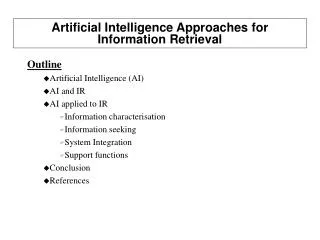
CS621: Artificial Intelligence. Pushpak Bhattacharyya CSE Dept., IIT Bombay Lecture 44– Multilayer Perceptron Training: Sigmoid Neuron; Backpropagation 9 th Nov, 2010. The Perceptron Model . Output = y. y = 1 for Σ w i x i >= θ = 0 otherwise. Threshold = θ. w 1. w n. W n-1.

E N D
CS621: Artificial Intelligence Pushpak BhattacharyyaCSE Dept., IIT Bombay Lecture 44– Multilayer Perceptron Training: Sigmoid Neuron; Backpropagation 9th Nov, 2010
The Perceptron Model . Output = y y = 1 for Σwixi >=θ = 0 otherwise Threshold = θ w1 wn Wn-1 x1 Xn-1
y 1 θ Σwixi
Perceptron Training Algorithm • Start with a random value of w ex: <0,0,0…> • Test for wxi > 0 If the test succeeds for i=1,2,…n then return w 3. Modify w, wnext = wprev + xfail
Limitations of perceptron • Non-linear separability is all pervading • Single perceptron does not have enough computing power • Eg: XOR cannot be computed by perceptron
Solutions • Tolerate error (Ex: pocket algorithm used by connectionist expert systems). • Try to get the best possible hyperplane using only perceptrons • Use higher dimension surfaces Ex: Degree - 2 surfaces like parabola • Use layered network
Pocket Algorithm • Algorithm evolved in 1985 – essentially uses PTA • Basic Idea: • Always preserve the best weight obtained so far in the “pocket” • Change weights, if found better (i.e. changed weights result in reduced error).
XOR using 2 layers • Non-LS function expressed as a linearly separable • function of individual linearly separable functions.
Example - XOR • = 0.5 w1=1 w2=1 Calculation of XOR x1x2 x1x2 Calculation of x1x2 • = 1 w1=-1 w2=1.5 x2 x1
Example - XOR • = 0.5 w1=1 w2=1 x1x2 1 1 x1x2 1.5 -1 -1 1.5 x2 x1
Some Terminology • A multilayer feedforward neural network has • Input layer • Output layer • Hidden layer (assists computation) Output units and hidden units are called computation units.
Training of the MLP • Multilayer Perceptron (MLP) • Question:- How to find weights for the hidden layers when no target output is available? • Credit assignment problem – to be solved by “Gradient Descent”
Can Linear Neurons Work? h2 h1 x2 x1
Note: The whole structure shown in earlier slide is reducible to a single neuron with given behavior Claim: A neuron with linear I-O behavior can’t compute X-OR. Proof: Considering all possible cases: [assuming 0.1 and 0.9 as the lower and upper thresholds] For (0,0), Zero class: For (0,1), One class:
For (1,0), One class: For (1,1), Zero class: These equations are inconsistent. Hence X-OR can’t be computed. Observations: • A linear neuron can’t compute X-OR. • A multilayer FFN with linear neurons is collapsible to a single linear neuron, hence no a additional power due to hidden layer. • Non-linearity is essential for power.
Training of the MLP • Multilayer Perceptron (MLP) • Question:- How to find weights for the hidden layers when no target output is available? • Credit assignment problem – to be solved by “Gradient Descent”
Gradient Descent Technique • Let E be the error at the output layer • ti = target output; oi = observed output • i is the index going over n neurons in the outermost layer • j is the index going over the p patterns (1 to p) • Ex: XOR:– p=4 and n=1
Weights in a FF NN m wmn • wmn is the weight of the connection from the nth neuron to the mth neuron • E vs surface is a complex surface in the space defined by the weights wij • gives the direction in which a movement of the operating point in the wmn co-ordinate space will result in maximum decrease in error n
Sigmoid neurons • Gradient Descent needs a derivative computation - not possible in perceptron due to the discontinuous step function used! Sigmoid neurons with easy-to-compute derivatives used! • Computing power comes from non-linearity of sigmoid function.
Training algorithm • Initialize weights to random values. • For input x = <xn,xn-1,…,x0>, modify weights as follows Target output = t, Observed output = o • Iterate until E < (threshold)
Observations Does the training technique support our intuition? • The larger the xi, larger is ∆wi • Error burden is borne by the weight values corresponding to large input values
Backpropagation algorithm …. Output layer (m o/p neurons) j wji • Fully connected feed forward network • Pure FF network (no jumping of connections over layers) …. i Hidden layers …. …. Input layer (n i/p neurons)
Backpropagation for hidden layers …. Output layer (m o/p neurons) k …. j Hidden layers …. i …. Input layer (n i/p neurons) kis propagated backwards to find value of j
General Backpropagation Rule • General weight updating rule: • Where for outermost layer for hidden layers
= 0.5 w1=1 w2=1 x1x2 1 1 x1x2 1.5 -1 -1 1.5 x2 x1 How does it work? • Input propagation forward and error propagation backward (e.g. XOR)