Download
1 / 23
230 likes | 404 Views
Tropospheric Signal Delay Corrections. Seth I. Gutman NOAA Earth System Research Laboratory Boulder, CO 80305 USA

E N D
Tropospheric Signal Delay Corrections Seth I. Gutman NOAA Earth System Research Laboratory Boulder, CO 80305 USA NOAA/LSU Workshop on Benefits to the NOAA Community of the National Height Modernization Program (NHMP) and The National Spatial Reference System (NSRS) Miami, Florida 18 September 2008
Introduction • Since the elimination of SA, atmospherically-induced signal delays dominate the GPS/GNSS error budget. • For high accuracy applications, the best way to mitigate the impact of these delays is to estimate them as free parameters in the calculation of the antenna position. • This usually requires short (< 50 km) baselines or long (> several hour) observation periods to resolve integer-cycle ambiguities and achieve the necessary vertical accuracy for the NHMP and NSRS.
Introduction • A possible alternative is to augment the GNSS observations with sufficiently accurate iono and tropo delay estimates to allow very rapid ambiguity resolution under virtually all weather conditions. • NOAA’s Space Weather Prediction Center (SWPC) now provides operational ionospheric delay estimates using a space weather model called USTEC. The uncertainty of this model is about 2 TEC units (see http://www.swpc.noaa.gov/ustec/images/index.html). • The remainder of this presentation will discuss strategies for providing RT/NRT tropospheric signal delay corrections for high accuracy vertical positioning.
Trop Delay Estimation Options • Predictive refractivity models based on climatology: • Hopfield • Saastamoinen • WASS • Analytical refractivity models based on observations: • Surface measurements of temperature, pressure and relative humidity • Numerical weather prediction models • Hybrid using all available observations e.g. NOAATrop
Predictive Models • Use predictions derived from the mean and normal ranges of (surface or upper-air) temperature, pressure and humidity. • “Climate is what you expect and weather is what you get.” Comparisons with independent SINEX solutions
Analytical Models • Use observations made at or interpolated to the location of the GNSS antenna. • Do well with the hydrostatic delay which uses Psfc with Saastamoinens’ zenith hydrostatic equation (1973). • Although the magnitude of the hydrostatic delay is 90-95% of the total tropospheric delay, ZHD is poorly correlated with ZTD.
Analytical Models (cont) • Use observations made at or interpolated to the location of the GNSS antenna. • Do poorly with the wet delay which use Tsfc and RHsfc with Saastamoinens’ zenith wet delay equation (1973). • This is because RHsfc is poorly correlated with the upper-air moisture that is responsible for most of the variability in ZTD.
Analytical Models (cont) • Use numerical weather prediction models that assimilate all available surface, upper-air and satellite observations. • Are more accurate in areas that have dense observations. • Generally do well estimating the zenith hydrostatic delay in areas of flat terrain. • All NWP models, especially those not assimilating GNSS observations) have difficulty with moisture. • In general, higher spatial resolution rapid-refresh models do better than lower resolution models under most circumstances.
Analytical Models (cont) • Use numerical weather prediction models that assimilate all available surface, upper-air and satellite observations. • NWP models assimilating GNSS water vapor observations analyze and predict atmospheric state variables (T, P, Q) much better than models not assimilating GNSS observations. Why? • GNSS observations provide accurate water vapor estimates under all weather conditions with high temporal resolution so they can effectively detect and monitor moisture variability.
NWP Model Without GNSS 13 6.5 0 -6.5 -13 32.5 26 19.5 13 6.5 0
NWP Model With GNSS 13 6.5 0 -6.5 -13 39 32.5 26 19.5 13 6.5 0
NOAATrop Model Animation courtesy of Sunil Bisnath (now at York University) and David Dodd, University of Southern Mississippi
Some Pertinent Questions • If GNSS-derived ZTD estimates improve NWP accuracy, can estimates of ZTD derived from atmospheric models improve PNT accuracy? • If so, by how much & under what conditions? • If not, why? • Some of these questions have been investigated by: • P. Alves, Y.W. Ahn, J. Liu, G. Lachapelle at U. Calgary; • S. Bisnath, D. Dodd at U. Southern Miss; • B. Remondi, M. Albright at XYZ’s of GPS; • F. Nievinski, M. Santos at U. New Brunswick; • Y. Bock and P. Fang at Scripps.
U. Calgary Results • Basic Technique > single reference station approach, a standard tropospheric model (Hopfield) and a robust ambiguity float solution = 15 - 25 cm • Multiple reference station approach = + 10-25% • Single reference station approach & = + 20-25% NOAATrop model • Combination of the multiple ref sta = + 27-40% approach & NOAATrop model
U. Southern Miss Results + 16.3% + 25.2% + 8.9%
Scripps Results • Running two CRTN networks in parallel: • Solve for 1 Hz 3-D positions and troposphere delay per site & compute 30-minute medians • One network: troposphere zenith delay constrained to 0.5 m, input nominal met values & Saastamoinen model • Second network: troposphere zenith delay constrained to 0.025 m, input NOAA model • With NOAA model: • Increase in position precision by ~15% • Increase in position accuracy by ~10% • NOAA model effectively reduces the correlation between zenith delay, multipath, and vertical position at all time scales, but impact diminishes with time.
Conclusions • All results are reasonably consistent. • The use of an analytical model such as NOAATrop adds value over predictive tropospheric delay models such as Saastamoinen, Hopfield and WASS. • XYZ’s of GPS reports that largest impacts occur during heavy precipitation. • Greatest improvements in vertical positioning accuracy in regions of significant terrain. • There are times when the NOAATrop model adds little value and can actually makes things worse. • Can we tell why this happens? • Can we tell when it’s happening?
When Does This Happen? • Problems manifest themselves in different ways: • In areas of high relief such as CA, RMS errors are associated with increased bias. • This suggests that the problem may be related to the spatial resolution of the model. • In areas of low relief and high moisture content, RMS errors are associated with increased standard deviation. • This suggests that the problem is related to the ability of the model to capture the spatiotemporal variability of moisture. • Ignoring horizontal gradients may be the cause.
Some Generalizations Moisture is relatively high along the Gulf Coast, variations occur rapidly on the scale of cloud fields Moisture is relatively low in the South West, and distribution is strongly controlled by topography. Model resolution is important. Horizontal gradients become more important
Recommendations • Establish NOAATrop model integrity monitors: • use local networks of CORS stations streaming RT data. • Compute single epoch solutions at high temporal frequency and compare with solutions using basic technique. • Broadcast “use NOAATrop” as long as solutions are better. • Broadcast “don’t use me I’m bad” as long as situation persists. • Use higher spatial resolution model in regions of high terrain. • Compute and use horizontal gradients. These can be generated directly from the NOAATrop model.