Woodhouse and Dziewonski, 1986

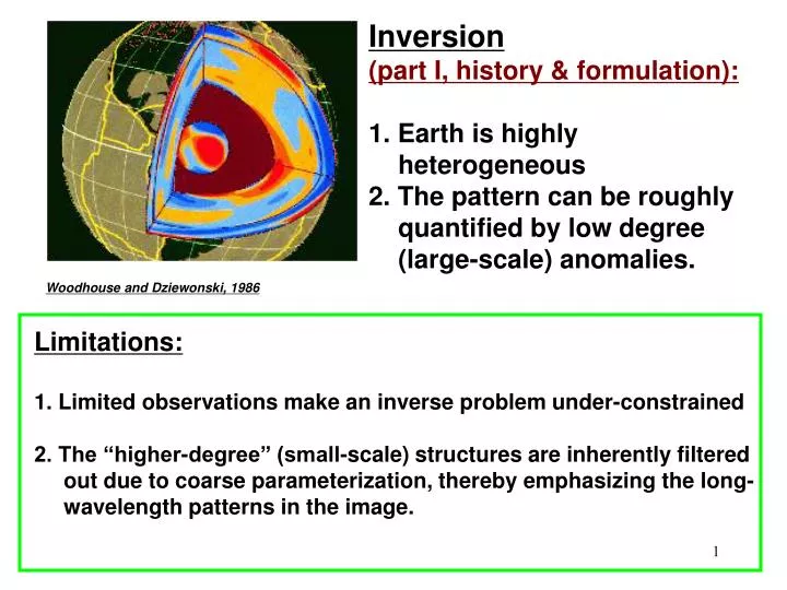
1. Inversion (part I, history & formulation): 1. Earth is highly heterogeneous 2. The pattern can be roughly quantified by low degree (large-scale) anomalies. Woodhouse and Dziewonski, 1986 Limitations: 1. Limited observations make an inverse problem under-constrained 2. The “higher-degree” (small-scale) structures are inherently filtered out due to coarse parameterization, thereby emphasizing the long-wavelength patterns in the image.

2. Mantle tomography • E.g., Bijwaard, Spakman, Engdahl, 1999. Subducting Farallon slab

3. History of Seismic Tomography Tomo— Greek for “tomos” (body), graphy --- study or subject Where it all began: Radon transform: (Johan Radon, 1917): integral of function over a straight line segment. Radon transform where p is the radon transform of f(x, y), and is a Dirac Delta Function (an infinite spike at 0 with an integral area of 1) p is also called sinogram, and it is a sine wave when f(x, y) is a point value.

4. Shepp-Logan Phantom (human cerebral) Radon Projected Input Recovered (output) Back projection of the function is a way to solve f() from p() (“Inversion”):

5. A few of the early medical tomo setups Fan beam, Multi-receiver, Moves in big steps Parallel beam Cunningham & Jurdy, 2000 Broader fan beam, Coupled, moving source receivers, fast moving Broader fan beam, Moving source, fixed receivers, fast moving (1976) Different “generations” of X-Ray Computed Tomography (angled beams are used to increase resolution). Moral: good coverage & cross-crossing rays a must in tomography (regardless of the kind)

6. Present Generation of models: Dense receiver sets, all rotating, great coverage and crossing rays. Brain Scanning Cool Fact: According to an earlier report, the best valentine’s gift to your love ones is a freshly taken brainogram. The spots of red shows your love, not your words!

7. Official Credit in Seismic Tomo: K. Aki and coauthors (1976) First tomographic study of california Eventually, something familiar & simple

8. Real Credit: John Backus & Free Gilbert (1968) First established the idea of Differential Kernels inside integral as a way to express dependency of changes in a given seismic quantity (e.g., time) to velocities/densities (use of Perturbation Theory). First “Global Seismic Tomographic Model” (1984) Freeman Gilbert Adam Dziewonski Don Anderson PREM 1D model (1981, Preliminary Reference Earth Model) ($500 K Crawford/Nobel Price) John Woodhouse Moral: Established the proper reference to express perturbations

9. Seismic Resolution Test (Checkerboard test) A seismic example with good coverage Input model: Top left Ray coverage: Top right Output model: Bottom right

12. y x Recipe Step 1: Linearize At the end of the day, write your data as a sum of some unknown coefficients multiply by the independent variable. Simple inverse problem: find intercept and slope of a linear trend. Slightly more difficult inverse problem: Cubic Polynomial Interpolation (governing equation)

13. Basis Functions and Construction of Data y x x x x x y y Weight=a3 y Weight=a1 y Weight=a4 Weight=a2

15. Travel time (or slowness) inversions: “sensitivity kernel”, Elements form an “A” matrix How to go from here? Solve for xijk (which are weights to the original basis functions). They corresponds to a unique representation of of seismic wave speed Perturbation. This process is often referred to as “Travel-time tomography”.

16. Least-Squares Solutions Suppose we have a simple set of linear equations A X = d We can define a simple scalar quantity E Mean square error (or total error) Error function We want to minimize the total error, to do so, find first derivative of function E and set to 0. So, do , we should have This is known as the system of normal equations. So this involves the inversion of the term ATA, This matrix is often called theinner-product matrix, or Toeplitz matrix. The solution is called the least-squares solution, while X=A-1 d is not a least squares solution.

17. Turning point (considered optimal) Goodness of fit m Pre-conditioning for ill-conditioned inverse problem (damping, smoothing, regularization. Purpose: Stabilize, enhance smoothness/simplicity) Lets use the same definition Define: An objective function J where where m is the damping or regularization parameter. Minimize the above by Left multiply by I is identity matrix (Damped Least Squares solution)

18. Errors are less severe in cases such as below A dense path coverage minimizes the amount of a priori information needed

19. Model Resolution (largesmall) Model Roughness (large small) Rawlinson et al., 2010 (PEPI)

20. Main Reasons for Damping, Purpose 1:Damping stabilizes the inversion process in case of a singular (or near singular matrix). Singular means the determinant = 0. Furthermore, keep in mind there is a slight difference between a singular A matrix and a singular ATA. A singular A matrix don’t always get a singular ATA. ATA inversion is more stable. In a mathematical sense, why more stable? Related to Pivoting - one can show that if the diagonal elements are too small, error is large (the reason for partial pivoting). Adding a factor to diagonal will help keep the problem stable. When adding to the diagonal of a given ATA matrix, the matrix condition is modified. As a result, A * X = d problem is also modified. So we no longer solve the original problem exactly, but a modified one depending on the size of m. We are sacrificing some accuracy for stability and for some desired properties in solution vector. Purpose 2: obtain some desired properties in the solution vector X. The most important property = smoothness.