Download
1 / 55
570 likes | 695 Views
Lateral Design. Lateral Material/Types. Drip tape Thin wall drip line Heavy wall drip line Polypipe with punch emitters Polypipe with sprays. Typical Layouts. More layouts. SDI. Lateral installation. SDI burial depth. Tape orientation One tape or more per bed Holes upward

E N D
Lateral Material/Types • Drip tape • Thin wall drip line • Heavy wall drip line • Polypipewith punch emitters • Polypipe with sprays
Tape orientation • One tape or more per bed • Holes upward • Tape thickness • Trend toward thicker • Tape materials • Stretch vs. breakage
Lateral Line Design • Important lateral characteristics • Flow rate • Location and spacing of manifolds • Inlet pressure • Pressure difference
Standard requires • Pipe sizes for mains, submains, and laterals shall maintain subunit (zone) emission uniformity (EU) within recommended limits • Systems shall be designed to provide discharge to any applicator in an irrigation subunit or zone operated simultaneously such that they will not exceed a total variation of 20 percent of the design discharge rate.
Design objective • Limit the pressure differential to maintain the desired EU and flow variation • What effects the pressure differential • Lateral length and diameter • Economics longer and smaller • Manifold location • slope
Allowable pressure loss (subunit) This applies to both the lateral and subunit. Most of the friction loss occurs in the first 40% of the lateral or manifold Ranges from 2 to 3 but generally considered to be 2.5 DPs =allowable pressure loss for subunit Pa = average emitter pressure Pn = minimum emitter pressure
Example Given: CV=0.03, 3 emitters per plant, qa = .43gph Pa=15 psi, EU=92, x=0.57 Find: qn, Pn, and P
Flow rate Where: l = Length of lateral, ft. (m). Se = spacing of emitters on the lateral, ft. (m). ne = number of emitters along the lateral. qa = average emitter flow rate, gph (L/h)
Manifold spacing • Spacing is a compromise between field geometry and lateral hydraulics • Lateral length is based on allowable pressure - head difference. • Have the same spacing throughout the field in all crops
Manifold Location • More efficient to place in middle • two laterals extend in opposite directions from a common inlet point on a manifold, they are referred to as a pair of laterals. • Manifold placed to equalize flow rates on the uphill and downhill laterals
Determine optimum lateral length • EU • Slope • Based on friction loss • limited to ½ the allowable pressure difference (ΔPs)
Hydraulics • Limited lateral losses to 0.5DPs • Equation for estimating • Darcy-Weisbach (best) • Hazen-Williams • Watters-Keller (easiest, used in NRCS manuals)
Hazen-Williams equation hf =friction loss (ft) F = multiple outlet factor Q = flow rate (gpm) C = friction coefficient D = inside diameter of the pipe (in) L = pipe length (ft)
Watters-Keller equation hf = friction loss (ft) K = constant (.00133 for pipe < 5” .00100 for > 5”) F = multiple outlet factor L = pipe length (ft) Q = flow rate (gpm) D = inside pipe diameter (in)
Or Or use equation Where Fe= equivalent length of lateral, ft) K = 0.711 for English units) B = Barb diameter, in D = Lateral diameter, in
Adjusted length L’ = adjusted lateral length (ft) L = lateral length (ft) Se = emitter spacing (ft) fe = barb loss (ft)
Barb loss • More companies are giving a Kdfactor now days
Example Given: lateral 1 diameter 0.50”, qave=1.5gpm,Barb diameter 0.10” lateral 2 diameter 0.50”, qave=1.5gpm, k=.25 Both laterals are 300’ long and emitter spacing is 4 ft Find: equivalent length for lateral 1 and hetotal for lateral 2
Solution Lateral 1 Lateral 2
Procedure • Step 1 - Select a length calculate the friction loss • Step 2 – adjust length to achieve desired pressure difference ( 0.5DHs)
Step 3 - adjust length to fit geometric conditions • Step 4 - Calculate final friction loss • Step 5 – Find inlet pressure • Step 6 – Find minimum pressure
Next step is to determine Δh • Paired Lateral • Single Lateral – • Slope conditions • S > 0 • S = 0 • Slope Conditions • S < 0 and –S > friction slope
Last condition • S < 0 and –S < Friction slope Which ever is greater
Find minimum lateral pressure • Where S > 0 or S=0 • Where S < 0 and –S < Friction slope • Where S < 0 and –S > friction slope