Download
1 / 24
240 likes | 527 Views
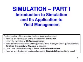
SIMULATION – PART I Introduction to Simulation and Its Application to Yield Management. For this portion of the session, the learning objectives are: Receive an introduction to the technique of Simulation . Learn the meaning of Yield Management .

E N D
SIMULATION – PART IIntroduction to Simulationand Its Application toYield Management • For this portion of the session, the learning objectives are: • Receive an introduction to the technique of Simulation. • Learn the meaning of Yield Management. • Illustrate how simulation can be applied to Yield Management in general and the Airplane Overbooking Problem in specific. • Learn how to simulate using a Table of Random Numbers. • Receive an introduction to simulation using Crystal Ball, an add-in to Excel.
GENERAL PRINCIPLES OF SIMULATION • A simulation is an experiment in which we attempt to understand how something will behave in reality by imitating its behavior in an artificial environment that approximates reality as closely as possible. (In this course, the artificial environment will be an Excel spreadsheet within a computer.) • Within this artificial environment, a simulation conducts an experiment that would be too costly and too time-consuming to conduct in reality. A simulation uses “funny money” and just a few minutes (or seconds) of time. • Because a simulation is based on random numbers, any value obtained from a simulation is only an estimate, that is, only an approximation of the true value. • Because a simulation is based on random numbers, obtaining accurate estimates requires a simulation with a very large number of “trials” (or “runs” or “iterations”). • Because a simulation requires a very large number of trials, a simulation is best conducted on a computer.
Yield Management is used by many businesses, such as: • Airlines • Hotels • Rental Cars • Restaurants Yield Management encompasses a wide variety of techniques, such as maximizing profit by determining how to adjust the prices of “seats” as it gets closer and closer to the date/time when customers will use the “seats”. In this course, we will not consider this technique. • A technique of Yield Management that we will consider is optimizing the number of reservations to confirm for a limited number of “seats”, where there are two types of penalties: • A penalty for having customers who have confirmed reservations but who are unable to “occupy a seat”, and • A penalty for having empty “seats” because of customers who are “no shows”. A common practice in Yield Management is overbooking, that is, confirming more reservations than the number of “seats” available. To illustrate how simulation can be applied to Yield Management, we will use an example of airplane overbooking.
EXAMPLE To illustrate both simulation and the airplane overbooking problem, we will consider the example below. NOTE: As indicated in Cell A13, we will temporarily assume that the maximum allowable number of confirmed reservations is 127.
SIMULATING DEMAND USING A TABLE OF RANDOM NUMBERS Random Numbers Corresponding to Demand Demand for Confirmed Reservations • As examples, • If RN = 07, then Demand = • If RN = 68, then Demand = • If RN = 83, then Demand =
The Binomial Probability Distribution • To model the scenario where customers with confirmed reservations are “no shows”, we will use the Binomial Probability Distribution. • Suppose there will be nindependent trials of an event that has two possible outcomes: • Outcome 1, with probability p • Outcome 2, with probability 1-p • Then, the number of the n trials that end in Outcome 1 has a Binomial Probability Distribution with parameters n and p. (Alternatively, the number of the n trials that end in Outcome 2 has a Binomial Probability Distribution with parameters n and 1-p.) • Example 1: The number of “heads” that results when you flip a coin 10 times has a Binomial Probability Distribution with parameters n=10 and p=0.50. • Example 2: If there is a 10% chance that a potential airplane passenger with a confirmed reservation is a “no show”, then the number of “no shows” that results when there are 120 confirmed reservations has a Binomial Probability Distribution with parameters n=120 and p=0.10. • For a Binomial Probability Distribution with parameters n and p, the mean is np and the variance is np(1-p). • The next slide displays the probability distributions for the Binomial Probability Distributions in Example 1 and Example 2 above.
Example 1: Flipping a Coin Example 2: “No Shows”
SIMULATION THE NUMBER OF “NO SHOWS” USING A TABLE OF RANDOM NUMBERS • For simplicity, assume • There 15 confirmed reservations. • 0.1 is the probability that a person with a confirmed reservation is a “No Show”. As examples, # of “No Shows” = # of “No Shows” = # of “No Shows” =
The following pages provide a summary of how to use Crystal Ball to analyze the Airplane Overbooking Problem.
OVERVIEW OF CRYSTAL BALL • After launching Crystal Ball, you will see the following menu and toolbars, where the three menu selections and the lower toolbar have been added-in to Excel. Crystal Ball permits three types of cells: • Assumption Cells: Each Assumption Cell contains a value about which you are uncertain. (Think of the Assumption Cells as the decision problem’s independent variables or inputs.) • Forecast Cells: Each Forecast Cell is one of the spreadsheet’s “bottom lines” and contains a formula that refers directly or indirectly to at least one of the Assumption Cells. (Think of the Forecast Cells as the decision problem’s dependent variables or outputs.) • Decision Cells: Each Decision Cell is under control of the decision maker and contains a value from of a set of alternative values. Copy Data Paste Data Run Preferences New Menu Selections Forecast Charts Create Report Define Forecast Start Simulation Define Decision Stop Simulation Single Step Define Assumption Reset Simulation
Defining Assumption Cell A18: the Demand for Confirmed Reservations The demand for confirmed reservations is a so-called Custom Probability Distribution. It would be too time-consuming to manually enter the Custom Probability Distribution displayed in the Cell Range R11:S60. Fortunately, Crystal Ball provides a way to “read in” the 50 values and the associated probabilities. To do so, we proceed as summarized on the next slide.
First click on Cell A18, next click the Define Assumption icon, then click Custom, and finally click OK. After doing so, the dialog box to the right appears. In this dialog box, first enter the Assumption Cell’s name as “Demand”, and then click LoadData. After doing so, the dialog box to the right appears. In this dialog box, enter the Cell Range R11:S60, and then click OK. After doing so, the dialog box to the right appears, in which the Custom Probability Distribution has been “read in”. Click OK to return to the spreadsheet.
Defining Assumption Cell A20: the Number of “No Show” Reservations • To define Assumption Cell A20, • Click on Cell A20. • Click Binomial. • Click OK. • In the resulting dialog box, • Enter the name as Number Who “No-Show”. • Enter “Probability” as the cell reference =A9, and enter “Trials” as cell reference =A19. • Click Enter. • Click OK.
After temporarily assuming that the maximum allowable of confirmed reservations is set to 127, after defining the two Assumption Cells in Cells A18 and A20, and after defining the Forecast Cell in Cell A27, we obtain the following spreadsheet: Our goal is to determine what value in Cell A13 will maximize the mean of Cell A27.
This slide and the following three slides display spreadsheets resulting from “debugging” the model by repeatedly clicking on the Single Step icon until four distinct types of scenarios are obtained. Scenario 1: Demand > Supply & Bumping Occurs
Now that we are confident that the spreadsheet has been properly constructed, we are ready to run the simulation. Recall that our goal is to determine the optimal value for the Maximum Number of Reservation to Confirm, that is the value for Cell A13 that maximizes the mean of the total contribution (to overhead and profit) Although time-consuming, one way to do this would be to run the simulation 35 times, first with Cell A13 =115, then with Cell A13 =116, …, and finally with Cell A13 =149. After doing so, we could then choose the value that maximized the mean of the total contribution. Wouldn’t it be nice if Crystal Ball could automate this process for us? In fact, Crystal Ball can do so through its Decision TableTool. The next slide illustrates how to use the Decision TableTool.
Using Crystal Ball’s Decision TableTool Step 1. To define the Decision Cell, first click cell and then click the Define Decision icon. The dialog box below will pop up. Within this box, enter a descriptive name for the decision and enter its lower & upper limits; then click on the radio button for Discrete and enter the Step. Finally click on OK. Step 2. Choose the Run, Tools, Decision Table menu selection. The dialog box below (#1 of 3) will pop up. Within this box, highlight one of the Forecast Cells to be the Target Cell (i.e., the Forecast Cell whose mean value you want to optimize). Then click Next. Step 3. In the resulting dialog box (#2 of 3), move the Decision Variable from “Available” to “Chosen” (i.e., from left to right) by first highlighting the decision variable and then clicking “>>”. Finally, click Next. Step 4. In the resulting dialog box (#3 of 3), first enter the number of trials for each simulation and then click Start.
Crystal Ball’s Decision Table Tool yields Rows 1-3 in the spreadsheet below. By clicking in Cell A1 on Forecast Charts, you can view any of the 35 Forecast Charts, including the one corresponding to the maximum Total Contribution, which can then be pasted into the spreadsheet.