Download
1 / 32
370 likes | 709 Views
Graph Codes and Expander Graphs. Coding Club presentation by Vitaly Skachek. Binary Symmetric Channel. Shannon Capacity of BSC where. 0. 0. p. p. 1. 1. Shannon Coding Theorem.

E N D
Graph Codesand Expander Graphs Coding Club presentation by Vitaly Skachek
Binary Symmetric Channel • Shannon Capacity of BSCwhere 0 0 p p 1 1 Graph Codes.
Shannon Coding Theorem • For any design rate R< thereexists an infinite family of codes satisfying the following conditions: • The length of approaches infinity with i growing. • The rate of satisfies for all i. • The decoding error probability under ML decoding decays exponentially with the length. Graph Codes.
LDPC Codes • Presented by R. Gallager in 1962. • Efficient decoding using belief propagation. • Performance at the rates below Shannon capacity. • Almost forgotten. • Turbo Codes • Berrou, Glavieux and Thitimajshima, 1993. • Empirically perform at rates very close to Shannon capacity. • Efficient encoding-decoding algorithms. • No exhaustive analysis. Graph Codes.
LDPC Codes • New interest in LDPC Codes. • Similarity between Turbo and LDPC. • Turbo decoding can be understood as belief propagation decoding (McEliece, MacKay, Cheng). • Main Results on LDPC Codes. • Good average behavior (Richardson, Urbanke). • Extremely close to the capacity codes were found by the exhaustive search (Richardson, Urbanke). • Explicit construction, constant fraction of correctable errors, linear encoding-decoding (Spielman). • Higher fraction of correctable errors (Zemor). Graph Codes.
Graph Codes • Proposed by Michael Tanner, 1981. • A special case of LDPC codes. Ingredients: • Internal -linear code • Bipartite graph Gwhere each node on some side of the graph has degree Graph Codes.
Bipartite Graph Presentation Sub-code Sub-code Check nodes 1 3 2 5 4 4 1 2 3 5 Variable nodes 2 0 1 0 2 1 Graph Codes.
Bipartite Graph Presentation Sub-code 1 2 3 4 5 Sub-code 1 2 3 4 5 1 0 2 0 1 2 1 0 1 2 Graph Codes.
Another Presentation Suppose that each variable node has degree equal 2. u v u v 0 0 The resulting graph is a graph with check nodes only. Each edge is labeled by the value of an appropriate bit. The labels on the edges incident to each node are codeword of Graph Codes.
Example Sub-code , generating matrix [ 1 0 1 ]. 1 1 0 0 1 1 The ordering of the edges incident to each node is important! 1 0 1 0 1 0 Graph Codes.
Lower Bound on the Rate Consider graph with |V| nodes. What is the rate of the resulting code? Each sub-code node contributes equations. Graph Codes.
Eigenvalues of the Graph • Let G be a ∆-regular connected non-trivial graph. Then ∆ is a largest eigenvalue of the adjacency matrix of G and an associated eigenvector is all-one vector. • If G is connected and bipartite then the smallest eigenvalue is -∆ and an associated eigenvector is a vector that has 1’s for entries of one side of the graph and –1’s for entries of the other side. • Let λbe a second largest eigenvalue. Then |λ|<∆. Graph Codes.
Second Eigenvalue • It is known that . • A graph G is called a Ramanujan graph if it is a connected ∆-regular graph such that every eigenvalue μ,, satisfies • Constructions by Lubotzky, Phillips, Sarnak and Margulis: for every integer ∆such that ∆-1 is a prime congruent to 1 modulo 4, there is an infinite sequence of arbitrarily large ∆-regular Ramanujan graphs (both bipartite and non-bipartite). Graph Codes.
Expander Graph • A ∆-regular graph G is called a c-expander if for every subset S of nodes • It could be shown that every ∆-regular graph G is a c-expander for • Intuition: in expander each subset of nodes has many neighbors (good expansion property). • Generally, smaller ratio yields better expansion and vice versa. Graph Codes.
Average Degree of Subgraph Lemma. Let G be a Δ-regular bipartite graph with vertex sets A and B where |A|=|B|=n and every edge has one endpoint in A and one point in B. Let S be a subset of A and T be a subset of B. The average degree of the subgraph induced by SUT satisfies Graph Codes.
Proof Let A be the 2nx2n adjacency vector matrix of the bipartite graph G. Let x be the column of length 2n such that every coordinate indexed by a vertex of S or of T equals 1 and the other coordinates equal 0. Graph Codes.
Proof Define : • Vector j– all ones vector. Eigenvector for ∆. • Vector k– vector that all coordinates indexed by A are 1 and all coordinates indexed by B are –1. Eigenvector for –∆. • Vector y Vector y is orthogonal to j and k. Graph Codes.
Proof We can write: Since , it follows that Graph Codes.
Proof Vector y is orthogonal to j and the eigenspace associated with the eigenvalue ∆ is of dimension one (G is connected and the matrix is symmetric). We have Substitution: Graph Codes.
number of entries value of entries |S| 1-|S|/n |T| 1-|T|/n n-|S| -|S|/n n-|T| -|T|/n Proof Computation of : Conclusion: Graph Codes.
Conclusion Graph Codes.
Expander Code 1 1 1 1 0 2 2 1 Sub-code C0of length Δ 0 1 0 0 A B 1 0 1 n 1 n Graph Codes.
Distance Bound Consider minimum weight non-zero codeword. 1 1 2 2 If some node has non-zero marked edge, it has at least such edges. Therefore, the average degree of the graph that contains such nodes is at least . n n Graph Codes.
Minimum Distance We showed that Suppose WLOG that . Then . Each node of T has at least non-zero incident edges. Therefore, Graph Codes.
D:maximum likelihood decoder for code ;: sub-codeword of z indexed by edges incident to the node v;m: number of iterations, will be discussed later. Input: Received word Let Fortomdo Ift odd thenX ← AelseX ← B Foreverydo Return z Decoding Graph Codes.
Expander Code 1 1 1 1 0 2 2 1 Sub-code C0of length Δ 0 1 0 0 A B 1 0 1 n 1 n Graph Codes.
Analysis Lemma. Suppose that . Let S be a subset of vertices of A such that where α<1. Let T be a subset of vertices of B and suppose that there exists a set Y of edges such that 1. every edge of Y has one endpoint in S; 2. every vertex of T is incident to at least edges of Y.Then Graph Codes.
Proof The graph has average degree greater or equal By the previous lemma Follows Since the result follows. Graph Codes.
Theorem Theorem. Suppose that . If the weight of the error vector x satisfies then the algorithms converges to the initial codeword. Key observation: if some node “sees” less than erroneous edges then all these edges will be corrected during the next iteration. Graph Codes.
Proof The number of erroneous nodes after the first iteration is upper-bounded by: On each further iteration, the number of erroneous nodes decreases exponentially. Graph Codes.
Complexity Analysis • During each round, the algorithm will construct a list of pointers to all constraints that could be unsatisfied. • During the first two iterations, the list contains pointers to all constraints. • On each further iteration, only nodes that have neighbors, which value was changes during the last iteration, could be unsatisfied. Graph Codes.
Complexity Analysis The amount of work to be done: Taking into account two first iterations, the overall time complexity is still bounded by O(N). Graph Codes.