Download
1 / 22
220 likes | 351 Views
Sample Data Analysis: Simple Regression. Enough theory (for now: more to come later!) To look at the data: type cd AFNI_data3/afni ; then afni Switch Underlay to dataset epi_r1 Then Axial Image and Graph FIM Pick Ideal ; then click afni/epi_r1_ideal.1D ; then Set

E N D
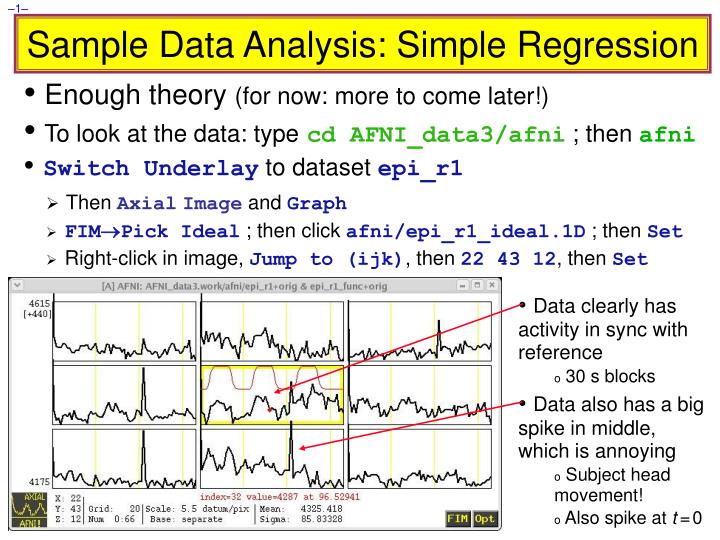
Sample Data Analysis: Simple Regression • Enough theory (for now: more to come later!) • To look at the data: typecd AFNI_data3/afni ; then afni • Switch Underlay to dataset epi_r1 • Then AxialImage and Graph • FIMPick Ideal ; then click afni/epi_r1_ideal.1D ; then Set • Right-click in image, Jump to (ijk), then 22 43 12, then Set • Data clearly has activity in sync with reference • 30 s blocks • Data also has a big spike in middle, which is annoying • Subject head movement! • Also spike at t=0
Preparing Data for Analysis • Six preparatory steps are common: • Temporal alignment: program 3dTshift • Image registration (AKA realignment): program 3dvolreg • Image smoothing: program 3dmerge • Image masking: 3dAutomask or 3dClipLevel • Conversion to percentile: programs 3dTstat and 3dcalc • Censoring out time points that are bad: program 3dToutcount (or 3dTqual) and 3dvolreg • Not all steps are necessary or desirable in any given case • In this first example, will only do registration, since the data obviously needs this correction
Data Analysis Script • 3dvolreg(3D image registration) will be covered in detail in a later presentation • filename to get estimated motion parameters • 3dDeconvolve = regression code • In file epi_r1_regress: 3dvolreg -base 3 \ -verb \ -prefix epi_r1_reg \ -1Dfile epi_r1_mot.1D \ epi_r1+orig 3dDeconvolve \ -input epi_r1_reg+orig \ -nfirst 3 \ -num_stimts 1 \ -stim_times 1 epi_r1_times.1D \ 'BLOCK(30)' \ -stim_label 1 AllStim \ -tout \ -bucket epi_r1_func \ -fitts epi_r1_fitts \ -xjpeg epi_r1_Xmat.jpg \ -x1D epi_r1_Xmat.x1D • Name of input dataset (from 3dvolreg) • Index of first sub-brick to process [skipping #0-2] • Number of input model time series • Name of input stimulus class timing file (’s) • and type of HRF model to fit • Name for results in AFNI menus • Indicates to output t-statistic for weights • Name of output “bucket” dataset (statistics) • Name of output model fit dataset • Name of image file to store X[AKA R] matrix • Name of text file in which to store X matrix • Type tcsh epi_r1_regress; then wait for programs to run
} MatrixQuality Assurance • 3dvolreg output • ++ 3dvolreg: AFNI version=AFNI_2007_05_29_1644 (Sep 5 2007) [64-bit] • ++ Reading input dataset ./epi_r1+orig.BRIK • ++ Edging: x=3 y=3 z=2 • ++ Initializing alignment base • ++ Starting final pass on 67 sub-bricks: 0..1..2..3.. *** ..63..64..65..66.. • ++ CPU time for realignment=5.35 s [=0.0799 s/sub-brick] • ++ Min : roll=-0.103 pitch=-1.594 yaw=-0.038 dS=-0.354 dL=-0.021 dP=-0.191 • ++ Mean: roll=-0.047 pitch=+0.061 yaw=+0.023 dS=+0.006 dL=+0.032 dP=-0.076 • ++ Max : roll=+0.065 pitch=+0.290 yaw=+0.055 dS=+0.050 dL=+0.120 dP=+0.113 • ++ Max displacement in automask = 2.46 (mm) at sub-brick 42 • ++ Wrote dataset to disk in ./epi_r1_reg+orig.BRIK • 3dDeconvolve output • ++3dDeconvolve: AFNI version=AFNI_2007_05_29_1644 (Sep 5 2007) [64-bit] • ++ Authored by: B. Douglas Ward, et al. • ++ loading dataset epi_r1_reg+orig • *+ WARNING: Input polort=1; Longest run=201.0 s; Recommended minimum polort=2 • ++ -stim_times using TR=3 seconds • ++ '-stim_times 1' using LOCAL times • ++ Wrote matrix image to file epi_r1_Xmat.jpg • ++ Wrote matrix values to file epi_r1_Xmat.x1D • ++ Signal+Baseline matrix condition [X] (64x3): 2.59165 ++ VERY GOOD ++ • ++ Signal-only matrix condition [X] (64x1): 1 ++ VERY GOOD ++ • ++ Baseline-only matrix condition [X] (64x2): 1.08449 ++ VERY GOOD ++ • ++ -polort-only matrix condition [X] (64x2): 1.08449 ++ VERY GOOD ++ • ++ Matrix inverse average error = 5.62791e-16 ++ VERY GOOD ++ • ++ Calculations starting; elapsed time=0.238 • ++ voxel loop:0123456789.0123456789.0123456789.0123456789.0123456789. • ++ Calculations finished; elapsed time=1.417 • ++ Wrote bucket dataset into ./epi_r1_func+orig.BRIK • ++ Wrote 3D+time dataset into ./epi_r1_fitts+orig.BRIK • ++ #Flops=3.11955e+08 Average Dot Product=4.50251 • If a program crashes, we’ll need to see this text output (at the very least)! Screen Output of the epi_r1_decon script }Maximum movement estimate } Consider '-polort 2' }Output file indicators }Progress meter/pacifier }Output file indicators
Stimulus Timing: Input and Visualization X matrix columns epi_r1_times.1D=9.0 69.0 129.0 =times of start of each BLOCK(30) HRF copy • HRFtiming • Linear in t • All ones aiv epi_r1_Xmat.jpg 1dplot -sepscl epi_r1_Xmat.x1D
Look at the Activation Map • Run afni to view what we’ve got (N.B.: a weak test with only 1 run) • Switch Underlay to epi_r1_reg (input for 3dDeconvolve) • Switch Overlay to epi_r1_func (output from 3dDeconvolve) • Sagittal Image and Graph viewers • FIMIgnore3 to have graph viewer not plot 1st 3 time pts • FIMPick Ideal; pick epi_r1_ideal.1D (modeled HRF: output from waver) • Define Overlay to set up functional coloring • OlayAllstim#0_Coef (sets coloring to be from model fit ) • ThrAllstim#0_Tstat (sets threshold to be model fit t-statistic) • See Overlay (otherwise won’t see the function!) – should be on automatically • Play with threshold slider to get a meaningful activation map (e.g., t =3 is a decent threshold — more on thresholds later) • Again, use Jump to (i j k) to jump to index coordinates 22 43 12
More Looking at the Results • Graph viewer: OptTran 1DDataset #N to plot the model fit dataset output by 3dDeconvolve • Will open the control panel for the Dataset #N plugin • Click first Input line to be ‘on’; then choose Dataset epi_r1_reg+orig • Also choose Color dk-blue to get a pleasing plot • Click 2nd Input on; then choose Dataset epi_r1_fitts+orig • Also choose Color limegreen to get a pleasing plot • Then click on Set+Close(to close the plugin’s control panel) • This tool lets you visualize the quality of the data fit • Can also now overlay function on MP-RAGE anatomical by using Switch Underlay to anat+orig dataset • Probably won’t want to graph the anat+orig dataset!
More Realistic Study • The Experiment • Cognitive Task: Subjects see photographs of two people interacting • The mode of communication falls in one of 3 categories: via telephone, email, or face-to-face. • The affect portrayed is either negative, positive, or neutral in nature. • Experimental Design: 3x3 Factorial design, BLOCKED trials • Factor A: CATEGORY - (1) Telephone, (2) E-mail, (3) Face-to-Face • Factor B: AFFECT - (1) Negative, (2) Positive, (3) Neutral • A random 30-second block of photographs for a task (ON), followed by a 30-second block of the control condition of scrambled photographs (OFF)... • Each run has 3 ON blocks, 3 OFF blocks. 9 runs in a scanning session.
Illustration of Stimulus Conditions AFFECT Negative Positive Neutral “You are the best project leader!” “Your project is lame, just like you!” “You finished the project.” Telephone CATEGORY "Your new haircut looks awesome!" "Ugh, your hair is hideous!" "You got a haircut." E-mail “I curse the day I met you!” “I feel lucky to have you in my life.” “I know who you are.” Face-to-Face • Data Collected • 1 Anatomical (MPRAGE) dataset for each subject • 124 axial slices • voxel dimensions = 0.938 x 0.938 x 1.2 mm • 9 Time Series (EPI) datasets for each subject • 34 axial slices x 67 volumes = 2278 slices per run • TR = 3 sec; voxel dimensions = 3.75 x 3.75 x 3.5 mm • Sample size, n=16 (all right handed)
Multiple Stimulus Classes • Summary of the experiment • 9 related communication stimulus types in a 3x3 design of Category by Affect (stimuli are shown to subject as pictures) • Telephone, Email & Face-to-face = categories • Negative, Positive & Neutral = affects • telephone stimuli: tneg, tpos, tneu • email stimuli: eneg, epos, eneu • face-to-face stimuli: fneg, fpos, fneu • Each stimulus type has 3 presentation blocks of 30 s duration • Scrambled pictures (baseline) are shown between blocks • 9 imaging runs, 64 useful time points in each • Originally, 67 TRs per run, but skip first 3 for MRI signal to reach steady state (i.e., eliminate initial transient spike in data) • So 576 TRs of data, in total (649) • Already registered and put together into one dataset: rall_vr+orig
Regression with Multiple Model Files • Script file rall_decon does the job: • Run this script by typing tcsh rall_regress (takes a few minutes) 3dDeconvolve -input rall_vr+orig \ -jobs 2 \ -concat '1D: 0 64 128 192 256 320 384 448 512' \ -num_stimts 15 -local_times \ -stim_times 1 '1D: 0 | | | 120 | | | | | 60' 'BLOCK(30)' \ -stim_times 2 '1D: * | | 120 | | 0 | | | | 120' 'BLOCK(30)' \ -stim_times 3 '1D: * | 120 | | 60 | | | | | 0' 'BLOCK(30)' \ -stim_times 4 '1D: 60 | | | | | 120 | 0 | |' 'BLOCK(30)' \ -stim_times 5 '1D: * | 60 | | 0 | | | 120 | |' 'BLOCK(30)' \ -stim_times 6 '1D: * | | 0 | | 60 | | | 60 |' 'BLOCK(30)' \ -stim_times 7 '1D: * | 0 | | | 120 | | 60 | |' 'BLOCK(30)' \ -stim_times 8 '1D: 120 | | | | | 60 | | 0 |' 'BLOCK(30)' \ -stim_times 9 '1D: * | | 60 | | | 0 | | 120 |' 'BLOCK(30)' \ -stim_label 1 tneg -stim_label 2 tpos -stim_label 3 tneu \ -stim_label 4 eneg -stim_label 5 epos -stim_label 6 eneu \ -stim_label 7 fneg -stim_label 8 fpos -stim_label 9 fneu \ • try to use 2 CPUs • run start indexes • stimulus times • '|' indicates new run • response model • stimulus label continued…
Regression with Multiple Model Files (continued) • motion regressor • apply to baseline -stim_file 10 motion.1D'[0]' -stim_base 10 \ -stim_file 11 motion.1D'[1]' -stim_base 11 \ -stim_file 12 motion.1D'[2]' -stim_base 12 \ -stim_file 13 motion.1D'[3]' -stim_base 13 \ -stim_file 14 motion.1D'[4]' -stim_base 14 \ -stim_file 15 motion.1D'[5]' -stim_base 15 \ -gltsym 'SYM: tpos -epos' -glt_label 1 TPvsEP \ -gltsym 'SYM: tpos -tneg' -glt_label 2 TPvsTNg \ -gltsym 'SYM: tpos tneu tneg -epos -eneu -eneg' \ -glt_label 3 TvsE \ -fout -tout \ -bucket rall_func -fitts rall_fitts \ -xjpeg rall_xmat.jpg -x1D rall_xmat.x1D • symbolic GLT • label the GLT • statistic types to output • 9 visual stimulus classes were given using -stim_times • important to include motion parameters as regressors? • this helps to exclude stimulus correlated motion artifacts • 6 motion parameters specified as covariates of no interest via -stim_file and -stim_base • 3dvolreg has previously been run, with the -1Dfile option, which gave us file motion.1D • can test the significance of the inclusion with –gltsym • Switch from -stim_base to -stim_label roll… • Use -gltsym 'SYM: roll \ pitch \yaw \dS \dL \dP'
} } Regressor Matrix for This Script (via -xjpeg) } Visual stimuli Baseline Motion • 18 baseline regressors • linear baseline • 9 runs times 2 params • 9 visual stimulus regressors • 33 design • 6 motion regressors • 3 rotations and 3 shifts aiv rall_xmat.jpg
Regressor Matrix for This Script (via -x1D) baseline regressors: via 1dplot -sepscl xmat_rall.x1D'[0..17]'
Regressor Matrix for This Script(via -x1D) • motion regressors • visual stimuli 1dplot -sepscl xmat_rall.x1D'[18..$]'
Options in 3dDeconvolve - 1 -concat '1D: 0 64 128 192 256 320 384 448 512' • “File” that indicates where distinct imaging runs start inside the input file • Numbers are the time indexes inside the dataset file for start of runs • In this case, a text format .1D file put directly on the command line • Could also be a filename, if you want to store that data externally -num_stimts 15 -local_times • We have 9 visual stimuli (+6 motion), so will need 9 -stim_times below • Times given in the -stim_times files are local to the start of each run (vs. -global_times meaning times are relative the start of the first run) -stim_times 1 '1D: 0.0 | | | 120.0 | | | | | 60.0' 'BLOCK(30)' • “File” with 9 lines, each line specifying the start time in seconds for the stimuli within the corresponding imaging run, with the time measured relative to the start of the imaging run itself (local time)
Aside: the 'BLOCK()' HRF Model • BLOCK(L) is convolution of square wave of duration L with “gamma variate function” (peak value=1 at t=4): • “Hidden” option: BLOCK5 replaces “4” with “5” in the above • Slightly more delayed rise and fall times • BLOCK(L,1) makes peak amplitude of block response=1 Black=BLOCK(30,1) Red=BLOCK5(30,1)
Options in 3dDeconvolve - 2 -gltsym 'SYM: tpos -epos' -glt_label 1 TPvsEP • GLTs are General Linear Tests • 3dDeconvolve provides test statistics for each regressor separately, but if you want to test combinations or contrasts of the weights in each voxel, you need the -gltsym option • Example above tests the difference between the weights for the Positive Telephone and the Positive Emailresponses • Starting with SYM: means symbolic input is on command line • Otherwise inputs will be read from a file • Symbolic names for each regressor taken from -stim_label options • Stimulus label can be preceded by + or - to indicate sign to use in combination of weights • Leave space after each label! • Goal is to test a linear combination of the weights • Tests if tpos =epos • e.g., does tpos get different response from epos ? • Quiz: what would 'SYM: tpos epos' test? It would test if tpos+ epos = 0
Options in 3dDeconvolve - 3 -gltsym 'SYM: tpos tneu tneg -epos -eneu -eneg' -glt_label 3 TvsE • Goal is to test if (tpos + tneu + tneg)–(epos + eneu + eneg)= 0 • Test average BOLD signal change among the 3 affects in the telephone tasks versus the email tasks -gltsym 'SYM: tpos -epos | tneu -eneu | tneg -eneg' -glt_label 3 TvsE_F • Goal is to test if tpos =epos, tneu =eneu, and tneg =enegare all true • BOLD signal change of any affect in the telephone tasks versus the email tasks • This is a different test than the previous one! • -glt_label 3 TvsEoption is used to attach a meaningful label to the resulting statistics sub-bricks • Output includes the ordered summation of the weights and the associated statistical parameters (t- and/or F-statistics) • t- or F-statistics?
Options in 3dDeconvolve - 4 -fout -tout = output both F- and t-statistics for each stimulus class (-fout) and stimulus coefficient (-tout)— but not for the baseline coefficients (if you want baseline statistics: -bout) • The full model statistic is an F-statistic that shows how well the sum of all 9 input model time series fits voxel time series data • Compared to how well just the baseline model time series fit the data times (in this example, have 24 baseline regressor columns in the matrix — 18 for the linear baseline, plus 6 for motion regressors) • F = [SSE(r)–SSE(f)]df(n) [SSE(f)df(d)] • The individual stimulus classes also will get individual F- and/or t-statistics indicating the significance of their individual incremental contributions to the data time series fit • e.g.,Ftpos (#6, equivalent to t (#5) ) tells if the full model explains more of the data variability than the model with tpos omitted and all other model components included • If DF=1, t is equivalent to F: t(n) = F2(1, n)
Results of rall_regress Script • Images showing results from third GLT contrast: TvsE • Menu showing labels from 3dDeconvolve run • Play with these results yourself!
Statistics from 3dDeconvolve • An F-statistic measures significance of how much a model component (stimulus class) reduced the variance (sum of squares) of data time series residual • After all the other model components were given their chance to reduce the variance • Residuals data – model fit = errors = -errts • A t-statistic sub-brick measures impact of one coefficient (of course, BLOCK has only one coefficient) • Full F measures how much the all regressors of interest combined reduced the variance over just the baseline regressors (sub-brick #0) • Individual partial-model Fs measures how much each individual signal regressor reduced data variance over the full model with that regressor excluded (e.g., sub-bricks #3, #6, #9) • The Coef sub-bricks are the weights (e.g., #1, #4, #7, #10) for the individual regressors • Also present: GLT coefficients and statistics Group Analysis: will be carried out on or GLT coefs from single-subject analyses