URBAN EMISSIONS AND PROJECTIONS

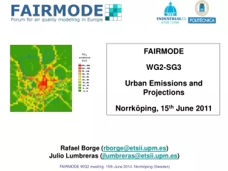
1. Parallel session FAIRMODE 2nd June 2010 URBAN EMISSIONS AND PROJECTIONS Rafael Borge1, Julio Lumbreras1, David de la Paz1, M. Encarnación Rodríguez1 Panagiota Dilara2, and Leonor Tarrason3 1 Laboratory of Environmental Modelling. Technical University of Madrid (UPM) 2 European Commission, Joint Research Centre, Ispra, Italy 3 Norwegian Institute for Air Research. Kjeller, Norway rborge@etsii.upm.es ; jlumbreras@etsii.upm.es

2. OUTLINE • Introduction • Methodology • Results • Conclusions

3. 1. Introduction FAIRMODE flowchart as agreed on 2nd plenary meeting (Nov. 2009)

4. SG(3) on urban emissions and projections • Background document on the emission needs at local scale • Needs for guidance on emission compilation at urban level • Consistency with national inventories • Top down vs bottom up approches • Use of GIS tools • Urban emission compilation is a key issue at European level • Both guidance and relevant exchange fora are needed • Next step: • Proposal for a framework for the development of emission inventories at local scale • Links to TFEIP/EIONET, NIAM, GEIA, JRC-EDGAR

5. assessment of ambient air quality planning and mitigation strategies Air Quality Modelling in the AQD assessment of the contribution of natural sources, road dust and sea salt short-term forecast for threshold exceedances • Uncertainties for Air Quality Models (AQMs) • Meteorology • Modelling system • Boundary and Initial conditions • Emission input • Uncertainties from emission inputs → emission inventories: • Emission data accuracy • Temporal disaggregation • Spatial resolution and emission allocation • Chemical speciation and mass distribution Consistent emission estimates across the scales, inventory harmonization. Criteria for local scale EI development

6. 1) Emission data accuracy (Cho et al., 2009) 2) Temporal disaggregation (Wang et al., 2010, Kühlwein et al., 2002) 3) Spatial resolution and emission allocation (Mensink et al., 2008, Cheng et al., 2008, Pisoni et al., 2010)

7. 2. Methodology • To analyse two approaches for different scale emission inventory compilation for an inland city and surroundings : • National calculation using country statistics and some regional data with spatial disaggregation afterwards • Regional calculation using regional data • Compare AQM results (whole year, 1-h resolution) with monitoring data • Select and analyse a number of representative stations where the alternative inventories produce important discrepancies in AQM results Relate these differences with emission compilation methods for the dominant source in the grid cell Understand reasons for discrepancies, get an idea about emission accuracy, and identify options for multi-scale emission inventory harmonization

8. AQM domain including AQ monitoring stations • Same BC and individual profiles for temporal and chemical speciation. Differences in model performance due to: • Emission data accuracy (total figures and sectoral figures) • Emission allocation (source apportionment at grid cell level)

9. Emission inventory aggregated comparison (INV1 – INV2) 3. Results

10. INV2 INV1 NOX emissions (t year-1) 10 • Emission allocation (Gridded total NOx emissions according to the inventories considered) • Largest discrepancies related to road transport and domestic/commcial/institut. heating • Some differences in industry-related combustion processes and off-road mobile sources • Different spatial allocation patterns

11. INV2 INV1 SNAP 02 contribution to NOX emissions at grid cell level (%) CAM 11 • Emission allocation: a) Source apportionment at grid cell level: SNAP 02 • Differences: • statistical basis used for activity rates estimation • population as spatial surrogate (uniform emission distribution across a given municipal urban area vs. CORINE land cover population density)

12. INV2 INV1 SNAP 07 contribution to NOX emissions at grid cell level (%) 12 • Emission allocation: b) Source apportionment at grid cell level: SNAP 07 • Differences: • discrepancies regarding driving patterns and road classification • differences in mileage estimation per vehicle (daily average intensities and road length vs. prescribed total mileage values depending on vehicle type) • road maps considered

13. 13 • AQM results: a) NO2 annual mean • AQM results: b) NO2 99.8th 1-h percentile

14. a INV1 INV2 b c INV1 INV2 INV1 INV2 14 • AQM results: c) NO2 Mean Bias (ppb) at station level Monitoring stations: A – traffic B – urban background C – industrial

15. Station A – INV1 Station A – INV2 15 • Station A (traffic) 2418 t/y 1093 t/y • INV1 more than double NOx emissions in the corresponding grid cell • SNAP 07 (road traffic) is the predominant source (consistent with station label) • INV2 considers a significant contribution from other sources • NO2 underestimated with INV2 and overestimated with INV1 similarly • Absolute mean errors (ME) and the correlation coefficient are similar • SNAP 07 emissions largely overestimated in INV1 (excessive contribution of heavy duty vehicles in highway driving patter), although activity ratios are more specific. • Inaccurate secondary EF

16. Station B – INV1 Station B – INV2 16 • Station B (urban background) 797 t/y 352 t/y • INV1 more than double NOx emissions in the corresponding grid cell • Source apportionment resulting in this grid cell is more balanced for INV2 • Non-LPS allocated using covers (INV2) and area-to-point algorithm (INV1) • NO2 slightly underestimated with INV2 and overestimated with INV1 • Better statistics for INV2 • SNAP 07 emissions overestimated in INV1 (dominating source in urban background) • Not enough information to support and area-to-point allocation strategy (spatial surrogates provide a more reasonable picture)

17. Station C – INV1 Station C – INV2 17 • Station C (industrial) 3616 t/y 672 t/y • INV1 more than triple NOx emissions in the corresponding grid cell • Road traffic emissions are in relatively good agreement • INV2 considers larger industrial emissions • NO2 overestimated with INV1 (MB = 14.8 ppb, ME = 20.3 ppb) • NO2 less underestimated with INV2 (MB = -3.6 ppb, ME = 12.6 ppb) • Apparently, an excessive emission allocation from industry in INV1 in general terms

18. Station C INV2 INV1 18 • Station 27 (industrial) • r coefficients similar • Important seasonal differences • Better agreement with observations during most of the year for INV2, except for particular periods concentrated in August-November • No significant differences in temporal patterns in those periods  • misrepresentations of the chemical split of NOx and VOCs for particular industrial activities • (most likely) high NO2 levels due to non-local contributions

19. 4. Conclusions • There is an increasing demand for high-resolution, fine-scale emission inventories for air quality modelling activities • It was agreed within FAIRMODE that this need is the most relevant emission-related issue for the application of the AQD • A reliable air quality model may be useful to discriminate the uncertainty of emission inventories • AQ monitoring sites should be carefully selected to guarantee the correctness and representativeness of the observational data considering the spatial and temporal resolution of the model • It is essential that the methodology used at different scales is known and transparent for all the inventories involved

20. Emissions from the road traffic are the key issue in an urban-scale inventory. Traffic flow measurements and accurate fleet characterization are crucial to get a reasonable estimate of traffic emissions. However, energy balances, computation methods and underlying hypotheses are, at least, equally important • A previous analysis of main statistics used to derived activity rates at different scales is needed. • The bottom-up approach is preferred when there is information enough to support a very detailed emission estimation, but a top-down approach in combination with an updated high-resolution land use/population cover may provide a more accurate picture of general emission distribution pattern. • If basic reference statistics are properly harmonised, both approaches should lead to quite similar results, being the differences due to the use of more specific information available only at finer scales

21. Laboratory of Environmental Modelling. Technical University of Madrid (UPM) THANK YOU FOR YOUR ATTENTION! rborge@etsii.upm.es ; jlumbreras@etsii.upm.es