Download
1 / 13
130 likes | 292 Views
Adaptive Hough transform for the search of periodic sources P. Astone, S. Frasca, C. Palomba Universita` di Roma “La Sapienza” and INFN Roma. Talk outline Hierarchical method for the blind search of periodic sources “Classic” Hough transform Non-stationarity Adaptive Hough transform

E N D
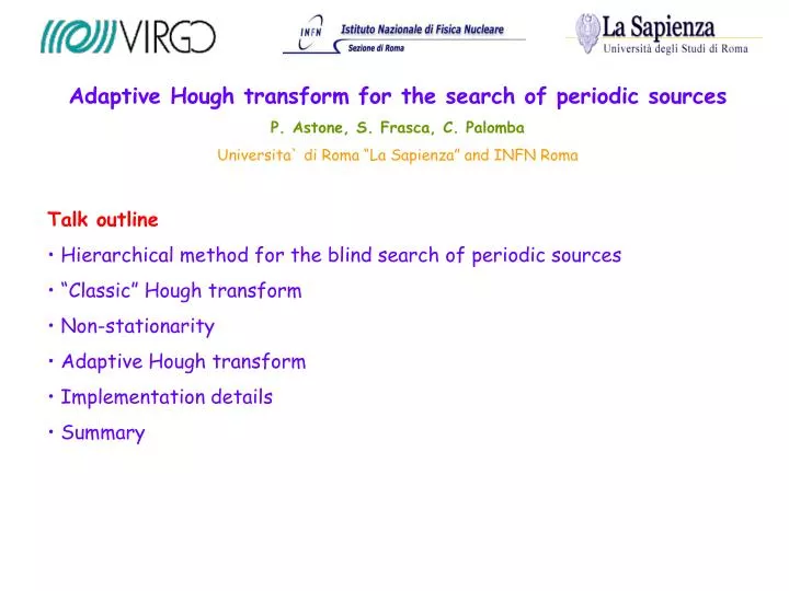
Adaptive Hough transform for the search of periodic sources P. Astone, S. Frasca, C. Palomba Universita` di Roma “La Sapienza” and INFN Roma • Talk outline • Hierarchical method for the blind search of periodic sources • “Classic” Hough transform • Non-stationarity • Adaptive Hough transform • Implementation details • Summary
Hierarchical method for the blind search of periodic sources h-reconstructed data SFDB SFDB The short FFT Database and the peak map for the hierarchical search of periodic sources P. Astone, S. Frasca, C. Palomba peak map peak map hough transf. hough transf. Evaluation of the sensitivity and of computing power for the Virgo hierarchical search P. Astone, S. Frasca, C. Palomba candidates coincidences candidates coherent step hough transf. events
“Classic” Hough transform It connects the time-frequency plane to the source parameter space. Each selected bin in the time-frequency peak map produces an ‘annulus’ of pixels in the Hough map, each set to one. A gravitational signal in the data produces a peculiar path in the time-frequency plane, due to the Doppler effect and the source spin-down. The ‘annuli’ corresponding to each signal peak intersect increasing the number count in a pixel of the Hough map corresponding to the source parameters. Tobs=4 months; SNR=0.01
The number count in a given pixel of the Hough map, built from N spectra, is given by • In absence of signals, the pixel number count is distributed according to a binomial distribution with • In presence of a signal the expected value is • where is the signal normalized power. if there is a peak contributing to that pixel in the i-th spectrum otherwise
Non-stationarity • Non-stationary disturbances: not predictable • Varying sensitivity pattern of the detector (with period of one sidereal day): • detector beam-pattern function generic detector matrix (interferometer: ) wave matrix in the detector reference frame
Adaptive Hough transform • How to take into account the non-stationarities? • For each spectrum we define a quantity • It is equal to one in the stationary case. • The noise is normalized before building the peak map, then the number of noise peaks is the same as in the stationary case, while the number of signal peaks is . • This is a consequence of for small signals. • We define Adaptive Hough Map the map in which the number count in a given pixel is • In absence of signals, the variance is • Let us normalize so that
If a signal is present, the number count in a given pixel of the map is which is maximizedif we take That is, we weight more the pixels which correspond to ‘good’ orientations of the detector and to less noisy spectra. • The number count distribution in the AHM is approximately gaussian. • The gain we have in using the AHM can be estimated comparing with the value of the number count obtained assuming to take the weights all equal:
Case I: amplitude modulation (circular polarization) In correspondence of the equatorial poles, the gain is 1 because there is no amplitude modulation • Case II: non-stationary noise (very ideal and simple case) r 1 A p 1
In this simple example the gain can be computed analitically as • From these two cases, we see that the gain in amplitude (the square root of the gain in the number count) is typically rather low and not larger than 20-30%. • This is a clear indication of the robustness of the Hough transform method, due to the fact that it uses peaks, and not the full spectral amplitude.
Implementative details • The weights corresponding to the detector beam pattern function are computed analytically once for all the pixels in the sky and for all the times; • The weights corresponding to non-stationary disturbances are computed before the Hough transform stage, using a low resolution power spectra, and are then used when the Hough map is built; • Each AHM is made of floats instead of short integers, then it memory occupancy is 2 times larger; • The computational weight increases of ~30% for the highest frequency band; it remains nearly the same for the lowest frequency band.
An example of AHM (beam pattern function taken into account) • The number count is reduced respect to the “classic” case; • The source ‘ghost’ image is strongly suppressed.
Summary • We have shown how to take into account non-stationarities in the computation of the Hough map; • In the adaptive Hough transform for each frequency bin contributing to a given pixel of the map, not 1 but a quantity proportional to the ‘amount’ of non-stationarity is summed; • The gain in using the AHM is not very large: typically 20-30% at most in amplitude. This is a clear indication of the robustness of the Hough transform method; • The computational weight increase up to ~30%; • The memory occupancy of AHM is increased by a factor of 2.