Download
1 / 22
220 likes | 226 Views
Economic growth theory: How does it help us to do applied growth work?. Elena Ianchovichina PRMED March 23, 2009. Why the focus on growth?. Most policymakers worry about growth and employment Yet, theory offers little advice on how to generate growth in a specific country

E N D
Economic growth theory:How does it help us to do applied growth work? Elena Ianchovichina PRMED March 23, 2009
Why the focus on growth? • Most policymakers worry about growth and employment • Yet, theory offers little advice on how to generate growth in a specific country • Growth is a fairly recent phenomenon in the period 1000-present • Large income differences between poor and rich countries • What can poor countries do to catch up? • What should rich countries do to maintain their high living standards?
Solow’s theory of growth • The centerpiece of Solow’s neoclassical model is the production function: Y=AF(K, L), where • Y is output, K is capital, L is labor, and A is a productivity parameter • Assuming CRS, we can rewrite the production function as: y=Af(k), where • y=Y/L (output per unit of labor), k=K/L (capital per unit of labor), and f(k)=F(k,1) • Output per capita y increases because of increases in capacity k and improvements in technology A
Emphasis on capital accumulationand strong assumptions • The neoclassical model emphasizes growth through capital accumulation: • where Iis investment, δ is the rate of capital depreciation • Expressing in units of labor and assuming that I=sY we have • where s is the saving rate, n is the rate of population growth, and all parameters are exogenous.
Economy in a steady state • In the steady state, the ratio of capital per unit of labor is stable: • or, using a “*” to denote a steady-state value, is determined by: • where is steady-state income y (n+δ)k y* sAf(k) k k*
Predictions I • The steady state rate of growth of real income per capita y depends only on g and does not depend on s or n • Real income Y grows at the rate of growth in technology and population (g+n) • If reform increases productivity, then income per capita would rise from y*(0) to y*(1) y sA1f(k) (n+δ)k y*(1) sA0f(k) y*(0) k k*
Predictions II • In the long run the economy approaches a steady state that is independent of initial k • In the steady state, k grows at the same rate as y, so k/y = s/(n+δ) • The steady state income y* depends on s and n. The higher s, the higher y*; the higher n, the lower y* y (n(2)+δ)k (n(0)+δ)k S(1)Af(k) y*(1) S(0)Af(k) y*(0) y*(2) k k*(2) k*(0) k*(1)
Predictions III • In the steady state, the marginal product of capital is constant • MP(K*)=(n+δ)/s=Af’(k*) • In the steady state, the marginal product of labor grows at the rate of technical change g • MP(L*)=A(f(k)-kf’(k)) • These predictions are broadly consistent with experience in the US
Critiques • Critique 1: model assumes technology is exogenous • We know income per capita grows as technology improves • Critique 2: countries use the same production function • Countries can be considered at different points on the same production function y (n1+δ)k (n2+δ)k y*(1) sAf(k) y*(2) k k*(2) k*(1)
Is the assumption of exogenous savings a problem? Not really • In the optimal growth literature savings are endogenously determined • Two basic approaches • In a OLG model (Samuelson and Diamond) • In a infinitely lived representative agent (Ramsey, Cass, Koopmans) • Both approaches yield results similar to Solow • The economy reaches a steady state with a constant saving rate • This steady state has the same characteristics as the steady state in the Solow model
From theory to empirics • Practical growth analysis has relied on • Growth accounting • Growth regressions • Macro models (e.g. CGE and others) • Complemented by microeconomic analyses at the firm level • What is the link between the neoclassical model and these techniques • The production function in Solow is the basis for these and other approaches
Growth accounting • Follows the standard Solow-style procedure to decompose output growth into contributions of capital K, labor L and productivity A • Production function represented for simplicity represented as a Cobb-Douglas function: • where is the share of capital in income. • Taking logs and time derivatives, leads to: • where “^” denotes percentage changes over time, capital growth consists of investment net of depreciation, and labor growth stands for the expansion of the working-age population • The production function in Solow is used to assess future potential growth output
Speed of convergence to steady state • In the Solow model income converges to its steady-state level at the same rate as capital: • where • is the capital share • The convergence equation holds for any type of production function
Cross country empirical analysis • Solow’s model is the basis for cross-country growth work as it predicts international income differences and conditional convergence • Steady-states differ by country depending on their rates of saving s and population growth n • Growth rates differ depending on country’s initial deviation from own steady state y A1y*(s1,n1) y1=A1f(k1) A2y*(s2,n2) y2=A2f(k2) t
Determinants of long-term growth • Cross-country growth regressions are used to assess the importance of the main factors determining steady state per capita • The literature is huge (Barro, 1995 and many others) • Three sets of factors are typically included in these regressions: • Structural policies and institutions • Education, financial depth, trade openness, government inefficiency, infrastructure, governance • Stabilization policies • Fiscal and monetary policies (inflation, cyclical volatility) • Monetary and exchange rate policies (real exchange rate overvaluation) • Regulatory framework for financial transactions • External conditions • Terms of trade shocks • Period specific shifts associated with changes in global conditions: recessions, booms, technological innovations
Cyclical output movements • Fatas (2002) shows that • Business cycles cannot be considered as temporary deviations from a trend • Countries with more volatile fluctuations display lower long-term growth rates y Ay*(s,n) y1=A1f(k1) t
Other approaches • Ramsey preceded Solow • Ramsey developed a rigorous yet very simple general-equilibrium model of optimal growth • This model offers an entry into the growth diagnostic approach of HRV (2005)
Simple Ramsey optimal growth model • Households have perfect foresight • Need to decide how much L and K to rent to firms, and how much to save or consume by maximizing their individual utility: • Subject to: • c is consumption per capita • n is population growth; • k is capital per worker; there is no depreciation • g is technological progress • θ is a distortion such as a tax • x is availability of complementary factors of productions • z is the rate of time preference
First-order conditions • Firms use CRS technology and maximize profits • Complementary factors x and taxes θare exogenous • First-order conditions for profit maximization imply: • Government spending is assumed to be fixed exogenously • Wages are given as w
Keynes-Ramsey rule • Maximizing (1) subject to (2) and (3), and carried out by setting up a Hamiltonian results in the following Keynes-Ramsey rule: • In this equation, σ is the elasticity of substitution between consumption at two points in time, t and s, and ρ(z) is the real interest rate • The Keynes-Ramsey rule implies that consumption increases, remains constant or declines depending on whether the marginal product of capital net of population growth exceeds, is equal to or is less than the rate of time preference • The larger the elasticity of substitution, the easier it is, in terms of utility, to forgo current consumption in order to increase consumption later for a given difference between the rate of return and the cost of capital
Keynes-Ramsey rule • In the case of balanced growth equilibrium: • The Keynes-Ramsey rule implies investment increases, remains constant or declines depending on whether the return to capital net of population growth exceeds, is equal to or less than the cost of capital • This equation is the starting point for the empirical HRV-type binding-constraints to growth analysis
Theory of second best • Welfare may decline if reforms tackling some distortions are implemented as long as other distortions remain • In formal terms, • u is welfare; τi is a distortion in activity i • λiis the Lagrange multiplier corresponding to the constraint associated with the distortion in activity i; • the distortion associated with the biggest multiplier effect is the binding constraint • represents the net marginal valuations of activityiby society s,and by private agents • The direct effect is always welfare improving, but the indirect effect may not be, implying that welfare may decline if the indirect effect is negative and larger than the direct effect