Download
1 / 32
320 likes | 433 Views
Two-Sample Proportions Inference. Two-Sample Proportions Inference. Sampling Distributions for the difference in proportions.

E N D
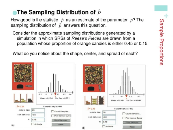
Sampling Distributions for the difference in proportions When tossing pennies, the probability of the coin landing on heads is 0.5. However, when spinning the coin, the probability of the coin landing on heads is 0.4. Let’s investigate. Pairs of students will be given pennies and assigned to either flip or spin the penny
Looking at the sampling distribution of the difference in sample proportions: What is the mean of the difference in sample proportions (flip - spin)? What is the standard deviation of the difference in sample proportions (flip - spin)? Can the sampling distribution of difference in sample proportions (flip - spin) be approximated by a normal distribution? What is the probability that the difference in proportions (flipped – spun) is at least .25? Yes, since n1p1=12.5, n1(1-p1)=12.5, n2p2=10, n2(1-p2)=15 – so all are at least 5)
Assumptions: • Two, independent SRS’s from populations ( or randomly assigned treatments) • Populations at least 10n • Normal approximation for both
The National Sleep Foundation asked a random sample of U.S. adults questions about their sleep habits. One of the questions asked about snoring. Of the 995 respondents, 37% of adults reported that they snored at least a few nights a week during the past year. Would you expect that percentage to be the same for all age groups? Split into two age categories, 26% of the 184 people under 30 snored, compared with 39% of the 811 in the older group. Is this difference of 13% real, or due only to natural fluctuations in the sample we’ve chose? HYPOTHESIS TEST! For the true DIFFERENCE between snoring rates!
Steps: • Assumptions • Hypothesis statements & define parameters • Calculations • Conclusion, in context
Assumptions: • Two, independent SRS’s from populations ( or randomly assigned treatments) • Populations at least 10n • Normal approximation for both
Assumptions: • Ages are independent of each other in random sample • 995 is less than 10% of all adults • Normal approximation for both
Hypothesis statements: H0: p1 - p2 = 0 Ha: p1 - p2 > 0 Ha: p1 - p2 < 0 Ha: p1 - p2 ≠ 0 H0: p1 = p2 Be sure to define both p1 & p2! Ha: p1 > p2 Ha: p1 < p2 Ha: p1 ≠ p2
Hypothesis statements: H0: There is no difference in snoring rates in the two age groups pold – pyoung = 0 p1= p2 Ha: There is a difference in snoring rates in the two age groups pold – pyoung ≠ 0 p1≠ p2
Since we assume that the population proportions are equal in the null hypothesis, the variances are equal. Therefore, we combine the variances!
Test statistic: Formula for Hypothesis test:
Test statistic: P-value = 2(area to right of z = 3.33) = .0008
Conclusion: “Since the p-value < (>) a, I reject (fail to reject) the H0. There is (is not) sufficient evidence to suggest that Ha.” Since the p-value is less that my significance level, I reject the null hypothesis of no difference. There is sufficient evidence to suggest that there is a difference in the rate of snoring between older adults and younger adults.
Formula for Hypothesis test: Usually p1 – p2 =0
Example - Student Retention A group of college students were asked what they thought the “issue of the day”. Without a pause the class almost to a person said “student retention”. The class then went out and obtained a random sample (questionable) and asked the question, “Do you plan on returning next year?” The responses along with the gender of the person responding are summarized in the following table. Test to see if the proportion of students planning on returning is the same for both genders at the 0.05 level of significance.
Example - Student Retention • Assumptions: • The two samples are independently chosen random samples. • Sample is less than 10% of college population. • The sample sizes are large enough since • n1 p1 =211 10, n1(1- p1) = 64 10 • n2p2 = 141 10, n2(1- p2) = 41 10 • so an approx normal model can be used. Significance level: = 0.05
Example - Student Retention pm = true proportion of males who plan on returning pf = true proportion of females who plan on returning nm = 275 (number of males surveyed) nf = 182 (number of females surveyed) (sample proportion of males who plan on returning) (sample proportion of females who plan on returning) Null hypothesis: H0: pm– pf = 0 Alternate hypothesis: Ha: pm – pf 0
Calculations: Test statistic:
P-value: The P-value for this test is 2 times the area under the z curve to the left of the computed z = -0.19. P-value = 2(0.4247) = 0.8494 Conclusion: Since P-value = 0.849 > 0.05 = , the hypothesis H0 is not rejected at significance level 0.05. There is no evidence that the return rate is different for males and females.
Example 4: A forest in Oregon has an infestation of spruce moths. In an effort to control the moth, one area has been regularly sprayed from airplanes. In this area, a random sample of 495 spruce trees showed that 81 had been killed by moths. A second nearby area receives no treatment. In this area, a random sample of 518 spruce trees showed that 92 had been killed by the moth. Do these data indicate that the proportion of spruce trees killed by the moth is different for these areas?
Assumptions: • Have 2 independent SRS of spruce trees • Both distributions are approximately normal since n1p1=81, n1(1-p1)=414, n2p2=92, n2(1-p2)=426 and all > 10 • Population of spruce trees is at least 10,130. H0: p1 = p2 where p1 is the true proportion of trees killed by moths Ha: p1 ≠ p2 in the treated area p2 is the true proportion of trees killed by moths in the untreated area P-value = 0.5547 a = 0.05 Since p-value > a, I fail to reject H0. There is not sufficient evidence to suggest that the proportion of spruce trees killed by the moth is different for these areas
CONFIDENCE INTERVAL! Back to snoring…. What if I wanted to know the true difference in the population proportion of young adults who snore and the proportion of older adults who snore? For the true DIFFERENCE between snoring rates!
What are the steps for performing a confidence interval? 1.) Identify the interval by name or formula (CI for two-sample proportion) 2.) Assumptions • Two, independent SRS’s from populations ( or randomly assigned treatments) • Populations at least 10n • Normal approximation for both 3.) Calculations 4.) Conclusion (in context of problem)
Formula for confidence interval: Margin of error! Standard error! Note: use p-hat when p is not known
Conditions for inference have previously been met Two-sample Confidence Interval for Proportions We are 95% confidence that the proportion of people who snore is between 5.92% and 20.28% higher for older adults than for younger adults.
Example 1: At Community Hospital, the burn center is experimenting with a new plasma compress treatment. A random sample of 316 patients with minor burns received the plasma compress treatment. Of these patients, it was found that 259 had no visible scars after treatment. Another random sample of 419 patients with minor burns received no plasma compress treatment. For this group, it was found that 94 had no visible scars after treatment. What is the shape & standard error of the sampling distribution of the difference in the proportions of people with no visible scars between the two groups? Since n1p1=259, n1(1-p1)=57, n2p2=94, n2(1-p2)=325 and all > 5, then the distribution of difference in proportions is approximately normal.
Example 1: At Community Hospital, the burn center is experimenting with a new plasma compress treatment. A random sample of 316 patients with minor burns received the plasma compress treatment. Of these patients, it was found that 259 had no visible scars after treatment. Another random sample of 419 patients with minor burns received no plasma compress treatment. For this group, it was found that 94 had no visible scars after treatment. What is a 95% confidence interval of the difference in proportion of people who had no visible scars between the plasma compress treatment & control group?
Assumptions: • Have 2 independent randomly assigned treatment groups • Both distributions are approximately normal since n1p1=259, n1(1-p1)=57, n2p2=94, n2(1-p2)=325 and all > 5 • Population of burn patients is at least 7350. Since these are all burn patients, we can add 316 + 419 = 735. If not the same – you MUST list separately. We are 95% confident that the true proportion of people who had no visible scars between the plasma compress treatment is between 53.7% and 65.4% higher than for the control group.
Example 2: Suppose that researchers want to estimate the difference in proportions of people who are against the death penalty in Texas & in California. If the two sample sizes are the same, what size sample is needed to be within 2% of the true difference at 90% confidence? Since both n’s are the same size, you have common denominators – so add! n = 3383
Do you think that the proportion of defective PEANUT M&Ms is higher than The proportion of defective PLAIN M&MS?