Presentation Outline

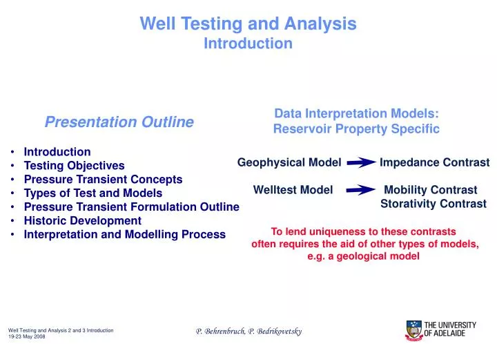
1. Data Interpretation Models: Reservoir Property Specific Geophysical Model Impedance Contrast Welltest Model Mobility Contrast Storativity Contrast Well Testing and Analysis Introduction Presentation Outline • Introduction • Testing Objectives • Pressure Transient Concepts • Types of Test and Models • Pressure Transient Formulation Outline • Historic Development • Interpretation and Modelling Process To lend uniqueness to these contrasts often requires the aid of other types of models, e.g. a geological model

2. Introduction

3. Investigations and Distances 1 cm 1 m 1 km Geology Seismic Cores Logs Static Distance of Investigation Formation Tester Welltests Tracers Dynamic 10-2 10-1 1 10 102 103 104 meter

4. What is Pressure Transient Testing? In a well test, the bottom hole pressure response (output), the result to a change in flow rate (input), is measured with a view to making important inferences regarding reservoir characteristics: thickness averaged permeability, conditions around the well bore (so called skin), reservoir limit, faults or any permeability barriers etc. That is why certain type of Well Testing may be equated to Pressure Transient Testing. To quantify the response we need a mathematical model of the reservoir: diffusivity equation. Output (response) Input (perturbation) Reservoir System (change in pressure) (change in q) matching Model input Mathematical Model Model output

5. Time Equates to Distance Production Rate Time • Near Well Effects (Early Time) • Afterflow • Skin (Impairment / Stimulation) • Homogeneous Reservoir (Mid-Time) • Permeability • Reservoir Fabric • Boundary / Drainage (Late Time) • Shape / Type (Boundary) • Volume Bottom Hole Pressure Time Increasing Time Reservoir Behaviour Boundary Effects Near Wellbore Effects

6. Testing Objectives

7. Well Testing • Controlled flow while measuring rates and pressures: • Drill Stem Test (DST) • For newly drilled wells: flowing through drill pipe • Production Test (PT) • For production wells: flowing through production tubing

8. A “Plan” for Well Testing • Reservoir description: • For planning a development • faults and barriers • natural fractures • layering • Reservoir evaluation: • For exploration and appraisal wells • production rate q • skin effect or near well bore damage (for PI calculation) • formation characteristics (kh) • reservoir limit testing • Reservoir management: • For development wells • monitoring average pressure for material balance calculations and forecasting • near well bore condition: work over or stimulation • (movement of) fluid fronts

9. Well Test Objectives • Commercial • Identification of type of fluid • Proving reserves • Establishing productivity • Technical • Reservoir characterisation • Average pressure • Average permeability • Inflow characteristics • Barriers/boundaries • Heterogeneity, eg. layers, fractures, etc • Flow rates • Completion design • Fluid sampling • Sand/ corrosion • Drive mechanism and depletion • Nearby gas cap • Aquifer (only for long term testing!)

10. What Can We Deduce? • Equilibrium Reservoir Pressure • - Material Balance - previous BHP’s ® Reservoir Drive • - Communication - RFT’s, BHP’s in other wells - Crossflow? • Transient Response of Reservoir • - Reservoir Transmissibility - Flow Characteristics • - Heterogeneity- Vertical- ‘Thief’ Zone? • - Areal- Proximal Boundary? • Transient Response of Well • - ‘Skin’ - Quantification of Impairment • - Reward for its removal • Semi - Steady State Response of Reservoir • - ‘Reservoir Limit Test’ - Drainage Volume • - Compressibility Drainage Area Simulator Aquifer

11. Pressure Transient Concepts

12. Well Testing Space, Time and Pressure Pi Transient Pressure Transient (A) Late Transient Semi-steady State Pwf (B) A (C) B Well linear C Time Transient (t < t4) Late Transient (t4 < t < t5) Pi t1 t2 t3 P t4 t5 First Boundary Last Boundary t6 r r = rw r = re

13. Types of Tests and Interpretation

14. Flow rate q BHP time The Most Common Tests Drawdown Results: e.g. permeability, skin, reservoir limit testing Pressure build up Flow rate q Results: e.g. permeability, skin, average drainage area pressure BHP time

15. Well Testing – Classification of Tests q q4 p p q3 Multi-Rate Test Pressure Drawdown q2 q1 t t q q p p Semi-Steady State Pressure Build-Up Reservoir Limit Test t t q Interference Test q Pulse Test

16. Well Testing Flow Geometry and Analysis Radial (Near Well) Log-Log Plot (Identification) Specialised Plot (Linear Trend) Radial (Near Well) linear linear Afterflow 45o Linear (Narrow Fault Block) linear linear ½ slope 45o

17. Well Testing Flow Geometry and Analysis (cont’d) Radial (Near Well) Log-Log Plot (Identification) Specialised Plot (Linear Trend) Hemi-spherical (Partial Penetration) linear Afterflow 45o Bi-linear (Hydraulic Fracture) linear ¼ slope linear linear ½ slope 45o

18. y y log x x log y log y x log x The Appearance of a pig seen through different mapping projections

19. Well Test Interpretation Model: More Degrees of Freedom Results in Non-uniqueness

20. Number and Meaning of Reservoir Parameters a Function of Interpretation Model

21. Pressure Transient Formulation Outline

22. Flow of an Incompressible Liquid through a Porous Medium Compared to Heat Conduction, Electro-statics and Current Conduction Permeability Dielectric constant Viscosity constant constant constant constant Source: Muskat, The Flow of Homogeneous Fluids through Porous Media, McGraw-Hill, 1937.

23. Pressure Transient Analysis Flow Chart for Governing Equations Modified Solutions Physical Relationships Modified Boundary Conditions Physical Assumptions Logarithmic Approximation (Used in Simplified Analyses) Diffusivity Equation Mathematical Assumptions Conditional Assumptions Linearised Diffusivity Eq. General Solution

24. Historic Development

25. Welltest Analysis Milestones

26. Welltest Analysis References

27. Data and Interpretation Technology Advances

28. The Paradigm Shift of the 1980s From A plethora of methods often giving different results To An integrated methodology based on a systems approach and signal theory

29. Analysis Techniques Power of Identification and Verification

30. Interpretation and Modelling Process

31. Well Test Interpretation: the Problem • This is an inverse problem: from the response of a system we infer the • properties of the system • With different (signal) input we may see very similar output (as in • history matching for reservoir simulation, material balance calculation) • This multiplicity is often due to lack of adequate information in • identifying a unique mathematical model • The number of unknowns always exceeds the number of equations – • hence follows the non-uniqueness • In conclusion: • Caution should be exercised in interpreting test results, • invoking all available information, for example core data

32. Well Test Interpretation Process Overview

33. Well Test Interpretation Process Details

34. Well Test Analysis: A Systems Approach

35. Well Test Analysis: Direct Problem I and S are Known: find O Convolution: unique solution Example: I = 2, 4, 6; S = S, O = 12 Application: model verification, well test design

36. Well Test Analysis: Inverse Problem 1 I and O are Known: find S Identification: non-unique solution Example: I = 2, 4, 6; O = 12, O = S or P Application: model diagnostics

37. Well Test Analysis: Inverse Problem 2 S and O are Known: find I Deconvolution: non-unique solution Example: O = 12; S = S, I = 1,11; 2,10; 3, 9; 4, 8; 5, 7; or 6, 6 Application: rate conversion

38. Interpretation Process (1) Model identification: a Pattern Recognition Problem Given the data, and knowing the characteristic shapes created by particular flow regimes, identify which flow regimes could create this type of data:

39. Interpretation Process (2) Model Parameter Calculation Given the data, interpret the same in a normal fashion:

40. Interpretation Process (3) Model Verification Given the data, and having identified a specific well test interpretation model as a possible solution, verify that the well test interpretation is consistent with the data:

41. Conversion factors useful in well testing and formation evaluation