Download
1 / 35
360 likes | 514 Views
From the ATLAS electromagnetic calorimeter to SUSY. Freiburg, 15/06/05 Dirk Zerwas LAL Orsay. Introduction ATLAS EM-LARG Electrons and Photons SUSY measurements Reconstruction of the fundamental parameters Conclusions. Introduction.

E N D
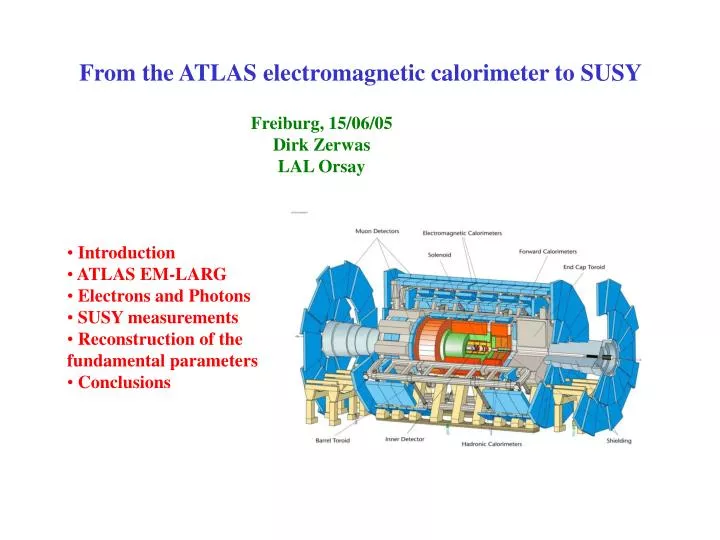
From the ATLAS electromagnetic calorimeter to SUSY Freiburg, 15/06/05 Dirk Zerwas LAL Orsay • Introduction • ATLAS EM-LARG • Electrons and Photons • SUSY measurements • Reconstruction of the • fundamental parameters • Conclusions
Introduction • LHC: CERN’s proton-proton colliderat 14TeV • 2800 bunchesof 1011 protons • bunch crossing frequency: 40.08MHz • Low Luminosity: 1033cm-2/s meaning 10fb-1 per experiment (3 years) • High Luminosity1034cm-2/s meaning 100fb-1 per experiment (n years) • SLHC: most likely 1035cm-2/s meaning 1000fb-1 per experiment (2015+) • startup for physics: late 2007 Two multipurpose detectors: ATLAS, CMS • Theexperimental challengesof the LHC environment: • bunch crossing every 25ns • 22events par BX (fast readout, 40MHz 200Hz, event-size 1.6MB) • High radiationFE electronics difficult (military and/or space technology) • and with that do precision physics!
Physicsat the LHC Process Events/s Events/year other machines Weν 15 108 104 LEP/ 107 TeV. Z ee 1.5 107 107 LEP tt 0.8 107 104 TeVatron bb 105 1012 108 Belle/Babar QCD jets 102 109 107 pT>200GeV You have heard already much about the physics from Sven Heinemeyer, Tilman Plehn, Christian Weiser,… plus in-house expertise on ATLAS-Tracker, ATLAS-Muons, Higgs physics,…..so try to find things of added value not covered so far: Calo+SUSYreco If the machine works well: Factory of Z, W, top and QCD jets. Will be limited quickly by systematics! • Measurements: • W mass to 20MeV needs control of the linearity/energy scale (0.02% energy scale) • Higgs mass measurement (if etc) in γγ • SUSY precision measurements with leptons • Stringent requirements on the energy scale, uniformity and linearity • of the ATLAS-EM Calorimeter response! Startup date getting closer, need to prove that we understand and are prepared Calo!
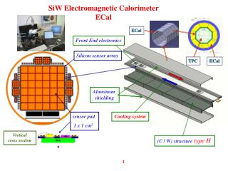
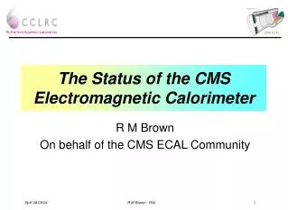
The ATLAS Electromagnetic Calorimeter • Liquid Argon Sampling Calorimeter: • lead (+s.s.) absorbers (1.1, 1.5mm Barrel) • liquid Argon gap 2.2mm 2kV (barrel) • varying gap and HV in the endcap • accordion structure no dead area in φ • “easy” to calibrate φ R 4m R 2.8m Z 0m Z 3.2m
The barrel and endcap EM-calorimeters! Some numbers: 2048 barrel absorbers 2048 barrel electrodes giving 32 barrel modules (4years of production and assembly) 16 endcap modules All assembled and inserted in their cryostats Barrel cryostat in pit waiting for electronics Barrel Thickness: 24-30X0 Granularity (typical Δη X Δφ ): Presampler = 0.025x0.1 (up to η=1.8) Strips = 0.003x0.1 (EC ) Middle = 0.025x0.025 (main energy dep) Back = 0.05 x0.025 Endcaps
Calibration of the ATLAS EM calorimeter • General Strategy and Sequence for electrons and photons: • Calibration of Electronics • necessitates a good understanding of the physics and calibration signal • Corrections at the cluster level: • position corrections • correction of local response variations • corrections for losses in upstream (Inner detector) material and longitudinal leakage • Refinement of corrections depending on the particle type (e/γ) • uniformity 0.7% with a local uniformity in ΔηXΔφ=0.2x0.4 better than 0.5% • inter-calibrate region with Zee • What can be studied where? • Calibration of electronics studied in testbeam • Corrections at cluster level: testbeam and ATLAS simulations • uniformity: testbeam • Zee: simulation • The best Monte Carlo is the DATA! For ATLAS: • Testbeam TestbeamMC ATLASMC ATLAS
ATLAS series modules in testbeam • 1998-2002: prototype and single module tests at CERN: • 4 ATLAS barrel modules • 3 ATLAS endcap modules • Single electron beams • 20-245GeV • Studies of: • energy resolution • linearity • uniformity • particle ID • 2004: combined testbeam endcap and barrel including tracking and muons FE electronics Sitting directly on the feedthrough as in ATLAS
The Signal/Electronics Calibration Preamp + shaper (3gains) + SCA Calibration signal : ~0.2% Physics signal • Electronics: • bipolar signal • time to peak 50ns (variable) • 40MHz sampling of 5 samples (125ns) • three gain system 1/9.5/10 • (automatic choice) 60 30 10 L (nH) • From 5 samples in time to one “energy”: • Optimal Filteringcoefficients: • exponential versus linear • different entry points • inductance effect: parallel versus serial • electronic gains L non-uniform: 2-3 % effect on E along 0 1.4
Digression:From physics to industry. Hamac SCA: Atlas Calorimeter Electronics. Sampling of 3x4 signals at 40MHz, 13.5 bits of dynamic range with simultaneous write and read in rad-hard technology (DMILL). Same type of chip used in digital oscilloscope: keep the high dynamic rangeand increase the sampling rate and bandwidth while using the cheapest technology on the market: 0.8µ pure CMOS (patent filed in April 2001). Instruments are based on the MATACQ chip which is a sampling matrix able to sample data at 2GS/s over 2560 points and 12 bits of dynamic range with a very low power consumption compared to standard systems. This structure has first been used in the design of the new digital oscilloscope family of Metrix (0X7000). This product is the first autonomous 12-bit scope on the market. Award for technology transfer to industry of the SFP (DPG) Also used in a 4-channel VME and GPIB board. The latter offers the 2GS/s – 12bits facility with low power at low cost. It’s perfectly suited for high dynamic range precise measurements in harsh environments (CAEN). Dominique Breton LAL-Orsay, Eric Delagnes CEA-Saclay
Cluster Corrections • Clustering with fixed size • Correct position S-shape in eta • Correct phi offset • S shape eta in strips • local energy variations phi (accordion) • local energy variations eta ATLAS simulation: S-shape Testbeam: phi modulation Endcap: Variation of correction as function of η under control (smooth behaviour)
Cluster Corrections: longitudinal weighting Non-negligeable amount of material before the calorimeter Reconstruction needs to optimise simultaneously energy resolution and linearity. Method based on Monte Carlo and tested with data in one pointη= 0.68: EPS = energy in presampler Ei =energy in calorimeter compartments Correct for energy loss upstream of Presampler (cryostat+beam line material) Energy lost between PS and calo (Cable/board) Small dependence of calo sampling fraction+ lateral leakage with energy Longitudinal leakage depth function of depth only 0.9 X0, 4.1 %@10 GeV 1.5 X0, 3.6 %@10 GeV > 30 X0, 0.3 %@10 GeV fbrem extracted from simulation and beam transport of H8 beam line, not present in ATLAS
Linearity • Dedicated setup was used in 2002 to have a very precise beam energy measurement : • - Degaussing cycle for the magnet to ensure B field reproducibility at • each energy (same hysteresis) • Use a precise Direct Current-Current Transformer with a precision of 0.01 % • Hall probe from ATLAS-Muon in magnet to cross-check magnet calibration • lots of help from EA-team (I. Efthymiopoulos) • Limitation of calorimeter linearity measurement is 0.03 % from beam energy knowledge • Absolute energy scale is not known in beam test to better than ~1 % • Relative variation is important • Achieved better than 0.1 % over 20-180 GeV but : • - done only at one position in a setup with less material than in ATLAS and no B field • No Presampler in Endcap (ATLAS) for >1.8 Systematics at low energy ~0.1 %
Energy resolution Resolution at =0.68 • Local energy resolution well understood since Module 0 beam tests and well reproduced by simulation : • Uniformity is at 1% level quasi online but achieving ATLAS goal (0.7 %) difficult Good agreement for longitudinal shower development between data and testbeam MC
Cluster Energy Corrections In ATLAS: use a simplified formula: E(corr) = Scale(eta)*(Offset(eta)+W0(eta)*EPS+E1+E2+W3(eta)*E3) 50GeV 3x7 10GeV 100GeV 0.1%-0.2% spread from 10GeV to 1TeV over all eta remember testbeam was 1point: proof that the method works!
Energy resolution in ATLAS Simulation Energy resolution in ATLAS wrt testbeam 20% worse Typically 2-4 X0 in front of calorimeter Good correlation with resolution Current method at the limit of its sensitivity For historians: wrt TDR 25% degradation, but in TDR simulation Inner Detector Material description incomplete 100GeV resolution X0 in front of strips
Barrel uniformity @ 245 GeV in testbeam rms 0.62% In beam setup, one feedthrough had quality problem ( open symbols) due to large resistive cross talk (non-ATLAS FT). > 7 is ATLAS like and can be used as reference : uniformity better than 0.5 % Energy scale differs by 0.13 % quality of module construction is excellent Module P13 0.45% Module P13 > 7 4.5‰ 0.49% Module P15 > 7 Module P13 Energy resolution Similar results for endcap modules
Position/Direction measurements in TB mid ~550 μm at =0 245 GeV Electrons strip ~250 μm at =0 sZ~20mm Hγγ vertex reconstructed with 2-3 cm accuracy in ATLAS in z Precision of theta measurement 50mrad/sqrt(E) sZ~5mm Good agreement of data and simulation
Zee • uniformity 0.2x0.4 ok in testbeam • description of testbeam data by Monte Carlo satisfactory • make use of Zee Monte Carlo and Data in ATLAS for intercalibration of regions • 448 regions in ATLAS (denoted by i) • mass of Z know precisely • Eireco = Eitrue(1+αi) • Mijreco =Mijtrue(1+(αi+αj)/2) • fit to reference distribution (Monte Carlo!!!) • beware of correlations, biases etc… At low (but nominal) luminosity, 0.3% of intercalibration can be achieved in a week (plus E/P later on)! Global constant term of 0.7% achievable!
Mass resolution of Higgs bosons H ZZ 4e: Mass scale correct within 0.1GeV σ=2.2GeV Hγγ 120.96GeV σ= 1.5GeV H γγ Note that the generated Higgs mass is 120GeV: Effect: calibration with electrons, so the photon calibration is off by 1-2% Getting from Electron to photon in ATLAS will require MC!
Particle Identification/jet rejection Dijet cross section ~1mb Z ee 1.5 10-6 mb W eν 1.5 10-5 mb Need a rejection factor of 105 for electrons Use the shower shape in the calorimeter Use the tracker Use the combination of the calo+tracker Cut based analysis gives for electrons an efficiency of about 75-80% with a rejection factor of 105 Multivariate techniques are being studied for possible improvements (likelihood, neural net, boost decision tree)
e id efficiency = 80% Pion rejection in: J/Psi : 1050±50 WH(bb) : 245±17 ttH : 166 ±6 Soft electrons • Two possibilities for seeded electron reconstruction • calo • tracker • Reconstruction of electrons close to jets difficult, and interesting (b-tagging) especially for soft electrons. Dedicated algorithm: • builds clusters around extrapolated impact point of the tracks • calculates properties of the clusters • PDF and neural net for ID • useful per se as well as for b-tagging Hbb pions J/Psi WH ttH What can we do now with all that?
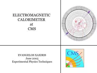
Supersymmetry See talks by Sven and Tilman: Here only a reminder for completeness sake 3 neutral Higgs bosons: h, A, H 1 charged Higgs boson: H± and supersymmetric particles: • The parameters of the Higgs sector: • mA : mass of the pseudoscalar Higgs boson • tanβ: ratio of vacuum expectation values • mass of the top quark • stop (tR, tL) sector: masses and mixing ~ ~ Theoretical limit: mh 140GeV/c2 ~ ~ ~ • Many different models: • MSSM (minimal supersymmetric extension SM) • mSUGRA (minimal supergravity) • GMSB • AMB • NMSSM ~ ~ • Conservation of R-parity • production of SUSY particules in pairs • (cascade) decays to the lightest sparticle • LSP stable and neutral: neutralino (χ1) • signature: missing ET
At the LHC Large cross section for squarks and gluinos of several pb, i.e. several kEvents sum jet-PT and ET effective mass Squarks and gluinos up to 2.5TeV “straight forward” Largest background for SUSY is SUSY (but…) SUSY SM Large masses means long decay chains Selection: multijet with large PT (typically 150,100,50 GeV) and OS-SF leptons Invariant masses jet-lepton, lepton-lepton, lepton-lepton-jet related to masses
SUSY at the LHC (and ILC) m0 = 100GeV m1/2 = 250GeV A0 = -100GeV tanβ =10 sign(μ)=+ favourable for LHC and ILC (Complementarity) Moderately heavy gluinos and squarks Heavy and light gauginos ~ • τ1 lighter than lightest χ± : • χ± BR 100% τν • χ2 BR 90% ττ • cascade: • qLχ2 q ℓR ℓq ℓℓqχ1 • visible ~ ~ ~ Higgs at the limit of LEP reach ~ light sleptons
Examples of measurements at LHC Gjelsten et al: ATLAS-PHYS-2004-007/29 From edges to masses: System overconstrained plus other mass differences and edges…
Using the kinematical formula (no use of model) and a toy MC for the correlated energy scale error: • energy scale leptons 0.1% • energy scale jets 1% • Mass determination for 300fb-1 (thus 2014): Coherent set of “measurements” for LHC (and ILC) “Physics Interplay of the LHC and ILC” Editor G. Weiglein hep-ph/0410364 Polesello et al: use of χ1 from ILC (high precision) in LHC analyses improves the mass determination
From Mass measurements to Parameters • SFITTER (R. Lafaye, T. Plehn, D. Z.): tool to determine supersymmetric parameters from measurements • Models: MSUGRA, MSSM, GMSB, AMB • The workhorses: • Mass spectrum generated by SUSPECT • (new version interfaced) or SOFTSUSY • Branching ratios by MSMLIB • NLO cross sections by Prospino2.0 • MINUIT • The Technique: • GRID (multidimensional to find a • non-biased seed, configurable) • subsequent FIT • Other approaches: • Fittino (P. Bechtle, K. Desch, P. Wienemann) • Interpolation (Polesello) • Analytical calculations • (Kneur et al, Kalinowski et al) • Hybrid (Porod) Beenakker et al
Results for MSUGRA Once a certain number of measurements are available, start with the most constrained model • Two separate questions: • do we find the right point? • need and unbiased starting point • what are the errors? • Convergence to central point • errors from LHC % • errors from ILC 0.1% • LHC+ILC: slight improvement • low mass scalars dominate m0 Sign(μ) fixed
Masses versus Edges Sign(μ) fixed • use of masses improves parameter determination! • edges to masses is not a simple “coordinate” transformation: Similar effect for m1/2 need correlations to obtain the ultimate precision from masses….
Total Error and down/up effect Theoretical errors (mixture of c2c and educated guess): Higgs error: Sven Heinemeyer et al. Including theory errors reduces sensitivity by an order of magnitude • Running down/up • spectrum generated by SUSPECT • fit with SOFTSUSY (B. Allanach) • central values shifted (natural) • m0 not compatible
Between MSUGRA and the MSSM • Start with MSUGRA, then loosen the unification criteria, • less restricted model defined at the GUT scale: • tanβ, A0, m1/2 , m0sleptons, m0squarks, mH2 , μ • experimental errors only Sfitter-team and Sabine Kraml • Higgs sector undetermined • only h (mZ) seen • slepton sector the same as MSUGRA • light scalars dominate determination of m0 • smaller degradation in other parameters, but still % precision The highest mass states do not contain the maximum information in the scalar sector, but they do in the Higgs sector!
MSSM With more measurements available: fit the low energy parameters LHC ILC LHC+ILC MSSM fit: bottom-up approach 24 parametersat the EW scale • LHC or ILC alone: • certains parameters must be fixed • LHC+ILC: • all parameters fitted • several parameters improved • Caveat: • LHC errors ~ theory errors • ILC errors << theory errors • SPA project: improvement of theory predictions and standardisation
Impact of TeVatron Data? Higgs mass from γγ • With Volker Buescher (Uni Freiburg): • 2008 too early for Higgs to γγ with 10fb-1 at LHC • only central cascade SUSY measurements are available: χ1, χ2, qL, ℓR • Higgs is sitting on the edge of LEP exclusion • WH+ZH 6 events per fb-1 and experiment at TeVatron • end of Run: Δmh = ± 2GeV • adding background: Δmh = ± 4-5GeV ~ ~ No Higgs, edges from the LHC: m0 = 100 ±14 GeV m1/2=250 ±10GeV tanβ= 10 ± 144 A0 = -100.37 ± 2400 GeV Higgs hint plus edges from the LHC: m0 = 100 ±9GeV m1/2=250± 9 GeV tanβ= 10 ±31 A0 = -100 ±685GeV • A hint of Higgs from the TeVatron would help the LHC at least the first year! • mtop from TeVatron with 2GeV precision makes impact on fit negligible
Stau coannihilation Wim de Boer: astro-ph/0408272 EGRET: on Compton gamma ray observatory, measured high energy gamma ray flux. Compatible with Standard Model, but also SUSY: m0 =1400 GeV m1/2 = 180 GeV A0=700 GeV tanβ = 51 μ > 0 0 mA resonance Stau LSP Dominant Processes at the LHC: Incomp. with EGRET data WMAP No EWSB Bulk EGRET And the Egret point? Tri-lepton signal promissing Les Houches 2005: P. Gris, L. Serin, L.Tompkins, D.Z. • Measurements: • Higgs masses h,H,A • mass difference χ2-χ1 • mass difference g- χ2 • Sufficient for MSUGRA m0=1400 ± (50 – 530)GeV m1/2 = 180 ± (2-12) GeV A0=700 ± (181-350) GeV tanβ= 51 ± (0.33-2) • Uncertainties: • b quark mass • t quark mass • Higgs mass prediction ~
Conclusions • Construction of ATLAS-EM calorimeter modules finished • Testbeam studies have driven the improvement of the understanding • of the combined optimisation of linearity and resolution of the calorimeter • EM calibration under control • electron (and photon identification) are at the required level • with multivariate approaches under study • SFitter (and Fittino) will be essential to determine SUSY’s fundamental • parameters • mass differences, edges and thresholds are more sensitive than masses • the LHC will be able to measure the parameters at the level % • LC will improve by a factor 10 • LHC+LC reduces the model dependence • EGRET: in MSUGRA, LHC has enough potential measurements to • confront the hypothesis • Many thanks to Laurent Serin for his help in the preparation of the talk!