Download
1 / 34
340 likes | 502 Views
Locating Internet Hosts. Venkata N. Padmanabhan Microsoft Research Harvard CS Colloquium 20 June 2001. Outline. Why is user or host positioning interesting? Two ends of the spectrum #1: RADAR: wireless LAN environment #2: IP2Geo: wide-area Internet environment Summary. Motivation.

E N D
Locating Internet Hosts Venkata N. Padmanabhan Microsoft Research Harvard CS Colloquium 20 June 2001
Outline • Why is user or host positioning interesting? • Two ends of the spectrum • #1: RADAR: wireless LAN environment • #2: IP2Geo: wide-area Internet environment • Summary
Motivation • Location-aware services help users interact better with their environment • Navigational services (inside a building, through city streets) • Resource location (nearest restaurant, nearest printer) • Targeted advertising (winter clothing, election canvassing) • Notification services (local events, weather alerts) • User positioning is a prerequisite to location-aware services • But this is a challenging problem
RADAR (Joint work with P. Bahl and A. Balachandran)
Background • Focuses on the indoor environment • Limitations of current solutions • global positioning system (GPS) does not work indoors • line-of-sight operation (e.g., IR-based Active Badge) • dedicated technology (e.g., ultrasound-based Active Bats) • RADAR goal: leverage existing infrastructure • use off-the-shelf RF-based wireless LAN • software adds value to wireless LAN hardware • better scalability and lower cost than dedicated technology
Basics • Key idea: signal strength matching • Offline calibration: • tabulate <location,SS> to construct radio map • empirical method or mathematical method • Real-time location & tracking: • extract SS from base station beacons • find table entry that best matches the measured SS • Benefits: • little additional cost • no line-of-sight restriction better scaling • autonomous operation user privacy maintained
Determining Location • Find nearest neighbor in signal space (NNSS) • default metric is Euclidean distance • Physical coordinates of NNSS user location • Refinement: k-NNSS • average the coordinates of k nearest neighbors N1, N2, N3: neighbors T: true location of user G: guess based on averaging
Experimental Setting • Digital RoamAbout (WaveLAN) • 2.4 GHz ISM band • 2 Mbps data rate • 3 base stations • 70x4 = 280 (x,y,d) tuples
RADAR Performance Median error distance is 2.94 m. Averaging (k=3) brings this down to 2.13 m
Dynamic RADAR System • Enhances the base system in several ways • mobile users • shifts in the radio environment • multiple radio channels • DRS incorporates new algorithms • continuous user tracking • environment profiling • channel switching
Continuous User Tracking • History-based model that captures physical constraints • used in cellular networks • Find the lowest cost path (à la Viterbi algorithm) • Addresses the problem of signal strength aliasing
Environment Profiling • Addresses problem of changing radio environment • System maintains multiple radio maps • Access points profile the environment and pick the best map
Summary of RADAR • RADAR: a software approach to user positioning • leverages existing wireless LAN infrastructure low cost • enables autonomous operation user privacy maintained • Base system • radio map constructed either empirically or mathematically • NNSS algorithm to match signal strength against the radio map • Enhanced system • continuous user tracking • environment profiling • Median error: ~2 meters • Publications: • Base system: INFOCOM 2000 paper • Enhanced system: Microsoft Technical Report MSR-TR-2000-12
IP2GEO (Joint work with L. Subramanian)
Background • Location-aware services are relevant in the Internet context too • targeted advertising • event notification • territorial rights management • Existing approaches: • user input: burdensome, error-prone • whois: manual updates, host may not be at registered location • Goal: estimate location based on client IP address • challenging problem because an IP address does not inherently indicate location
IP2Geo Multi-pronged approach that exploits various “properties” of the Internet • DNS names of router interfaces often indicate location • Network delay tends to increase with geographic distance • Hosts that are aggregated for the purposes of Internet routing also tend to be clustered geographically • GeoTrack • determine location of closest router with recognizable DNS name • GeoPing • use delay measurements to triangulate location • GeoCluster • extrapolate partial IP-to-location mapping information using cluster information derived from BGP routing data
Delay-based Location Estimation • Delay-based triangulation is conceptually simple • delay distance • distance from 3 or more non-collinear points location • But there are practical difficulties • network path may be circuitous • transmission & queuing delays may corrupt delay estimate • one-way delay is hard to measure • one-way delay round-trip delay/2 because of routing asymmetry
A 20 ms C 30 ms 10 ms T B
GeoPing • Measure the network delay to the target host from several geographically distributed probes • typically more than 3 probes are used • round-trip delay measured using ping utility • small-sized packets transmission delay is negligible • pick minimum among several delay samples • Nearest Neighbor in Delay Space (NNDS) • construct a delay map containing (delay vector,location) tuples • given a vector of delay measurements, search through the delay map for the NNDS • location of the NNDS is our estimate for the location of the target host
4000 km 1 10 5 11 12 6 2 13 7 14 3 2000 km 4 8 9 Redmond, WA Madison, WI Austin, TX Durham, NC 1 5 9 13 Berkeley, CA Urbana, IL Boston, MA Chapel Hill, NC 2 6 10 14 Stanford, CA St. Louis, MO New Brunswick, NJ 3 7 11 Baltimore, MD San Diego, CA Dallas, TX 4 8 12 Delay map constructed using measured delays to 265 hosts on university campuses
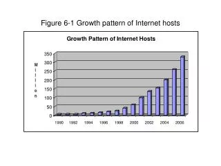
Validation of Delay-based Approach Delay tends to increase with geographic distance
Performance of GeoPing 9 probes used. Error distance: 177 km (25th), 382 km (50th), 1009 km (75th)
Performance of GeoPing Highest accuracy when 7-9 probes are used
GeoCluster • A very different approach from GeoPing • Basic idea: • divide up the space of IP addresses into clusters • extrapolate partial IP-to-location mapping information to assign a location to each cluster • given a target IP address, first find the matching cluster using longest-prefix match. • location of matching cluster is our estimate of host location • Example: • consider the cluster 128.95.0.0/16 (containing 65536 IP addresses) • suppose we know that the location corresponding to a few IP addresses in this cluster is Seattle • then given a new address, say 128.95.4.5, we deduce that it is likely to be in Seattle too
Clustering IP addresses • Exploit the hierarchical nature of Internet routing • we use the approach proposed by Krishnamurthy & Wang (SIGCOMM 2000) • inter-domain routing in the Internet uses the Border Gateway Protocol (BGP) • BGP operates on address aggregates • we treat these aggregates as clusters • in all we had about 100,000 clusters of different sizes
IP-to-location Mapping • Key points: • partial information, i.e., only for a small subset of addresses • not necessarily accurate • We obtained this from a variety of sources • FooMail: combined anonymized user registration information with client IP address • FooHost: derived location information from cookies • FooTV: combined zip code submitted in user query with client IP address
Extrapolating IP-to-location Mapping • Determine location most likely to correspond to a cluster • majority polling • “average” location • the dispersion is an indicator of our confidence in the location estimate • What if large geographic spread in locations? • some clusters correspond to large ISPs and the internal subdivisions are not visible at the BGP level • we have developed a novel sub-clustering algorithm to address this • some clients connect via proxies or firewalls (e.g., AOL clients) • use knowledge of dispersion to avoid making any location estimate at all
Performance of GeoCluster Median error: GeoTrack: 108 km, GeoPing: 382 km, GeoCluster: 28 km
Summary of IP2Geo • A variety of techniques that depend on different sources of information • GeoTrack: DNS names • GeoPing: network delay • GeoCluster: address aggregates used for routing • Median error varies 20-400 km • Even a 30% success rate is useful especially since we can tell when the estimate is likely to be accurate • Microsoft Technical Report MSR-TR-2000-110
Conclusions • RADAR and IP2Geo try to solve the same problem in very different contexts • wireless versus wireline • indoor environment versus global scale • accuracy of a few meters versus tens or hundreds of kilometers • Interesting but challenging problem! • For more information visit: http://www.research.microsoft.com/~padmanab/