TRENDS IN THE ELEMENTAL COMPOSITION OF PM2.5 IN SANTIAGO, CHILE FROM 1998 TO 2006

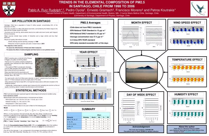
1. TRENDS IN THE ELEMENTAL COMPOSITION OF PM2.5 IN SANTIAGO, CHILE FROM 1998 TO 2006 Pablo A. Ruiz Rudolph*,†, Pedro Oyola†, Ernesto Gramsch‡, Francisco Moreno‡ and Petros Koutrakis* * Harvard School of Public Health, Department of Environmental Health, Boston, MA; † Centro Mario Molina Chile, Santiago, Chile ‡University of Santiago, Department of Physics, Santiago, Chile AIR POLLUTION IN SANTIAGO PM2.5 Averages MONTH EFFECT WIND SPEED EFFECT • Santiago, Chile has a population of about 6 million people, concentrating 40% of the population of Chile. • The city is located in a valley (520 above sea level), surrounded by the Andes range to the East and the Coastal range to the West • Summers are hot and dry, while winters tend to be colder and more humid, with frequent thermal inversions. • Major sources include large number of industries and a large vehicle and bus fleet (800,000) • Recent air quality interventions include: • Street cleaning and tree planting campaign in 1998 • Reduction of lead in gasoline and sulfur in diesel fuels in 2001 • The objective of this work is: • To asses the effectiveness of these and other measures • To assess the effect of meteorological and time factors on air pollution levels • Chile does not have PM2.5 standards • EPA National YEAR Standard is 15 μgr m-3 • EPA National DAILY standard is 35 μgr m-3 • Average concentration was 37.4 μgr m-3 • 2.5 times EPA YEAR standard • EPA daily standard exceeded 40% of the days YEAR EFFECT SAMPLING • PM2.5 sampling was conducted at the Parque O’Higgins air quality monitoring station • Twenty-four hour particle samples (midnight to midnight) were collected from April 1998 through March 2006 • Fine particle (PM2.5, aerodynamic diameter <2.5 μm) filter samples were collected on Teflon filters using dichotomous samplers • Mass was determined by gravimetry and elements by X-ray fluorescence (Desert Research Institute, Reno, NV, USA) TEMPERATURE EFFECT • For each month, only 6 to 8 filters were selected, or about 1 sample every fourth day, for a total of 717 filters analyzed across the eight years of the study • Only elements that had at least 80% of all reported values above LOD were included in the statistical analysis • Additionally, meteorological variables were measured at the sampling site and the La Paz air quality monitoring station, located a few kilometers north/northwest. STATISTICAL METHODS HUMIDITY EFFECT • PM2.5 and elements were regressed against meteorological and temporal variables using linear regression models • Meteorological data were dichotomized or trichotomized as follows: • Wind speed (ws), ws < 0.8 m/s, 0.8 ≥ ws< 1.6 m/s, ws ≥ 1.6 m • Relative humidity, rh < 70% and rh≥70% • Temperature t < 20oC and t ≥ 20oC • Years were counted from April of one year to March of the following year • Model • Where, α is the regression intercept and βyj, βmj, βwj, βwsj, βtmpj, and βrhj are the regression coefficients of the independent variables year (1 to 8), month (1 to 12), weekday (1 to 7), wind speed (1 to 3), temperature (1 to 2) and relative humidity (1 to 2) • As exponential terms: • [PM] = I * fyearj * fmonthj * fweekdayj * fwsj * ftmpj * frhj • Fij are the Concentration Impact Factor (CIF). CIFs are multiplicative rather than additive. I.e. a CIF of 2 for June means concentrations in January are twice the concentrations in December • The CIF for the intercept, I = eα, corresponds to the average concentration at the reference level (e.g. Year 2006, December, Saturday, ws ≥ 1.6 m/s, rh ≥70% and tmp ≥ 20 oC) DAY OF WEEK EFFECT SUMMARY Acknowledgement This work was funded by CONAMA RM The authors want to thank SESMA for sample collection About the author Pablo Ruiz is a Research Fellow at HSPH and a Research Associate at Centro Mario Molina Chile Contact at email pruiz@hsph.harvard.edu