Download
1 / 32
320 likes | 663 Views
Open-Economy Macroeconomics: The Balance of Payments and Exchange Rates. CHAPTER OUTLINE. The Balance of Payments Equilibrium Output (Income) in an Open Economy The Open Economy with Flexible Exchange Rates. Adapted from:. Fernando & Yvonn Quijano. 20.1 Introduction.

E N D
Open-Economy Macroeconomics: The Balance of Payments and Exchange Rates CHAPTER OUTLINE The Balance of Payments Equilibrium Output (Income) in an Open Economy The Open Economy with Flexible Exchange Rates Adapted from: Fernando & Yvonn Quijano
20.1 Introduction International trade is a major part of today’s world economy. When people in different countries buy from and sell to each other, an exchange of currencies must also take place. The main difference between a domestic transaction and an international transaction concerns currency exchange. The former uses a single currency while the latter uses several difference currencies. For instance, when Malaysia imports machinery from the U.S., the standard currency is the U.S. dollars (U$). In the above case, the exchange rate of MYR/U$ will determine the costs of imported goods. If the rate goes up from MYR3/U$ to MYR4/U$, the Malaysian importer will have to pay MYR4000 for a U$1000 machine (compared with MYR3000 before the rate increases).
Early in the century, during the gold standard era, nearly all currencies were backed by gold. The values were fixed in terms of a specific number of ounces of gold. At the end of World War II, the Bretton Woods system came into force before its demise in 1971. Under this system, countries were to maintain fixed exchange rates with each other. Governments must at times intervene to keep currencies aligned at their established values. After 1971, exchange rates are determined essentially by supply and demand, either under a freely floating system (no government intervention) or managed floating system (limited intervention). foreign exchange All currencies other than the domestic currency of a given country.
20.2 The Balance of Payments • balance of payments The record of a country’s transactions in goods, services, and assets with the rest of the world; also the record of a country’s sources (supply) and uses (demand) of foreign exchange. • The balance of payments is divided into 2 major accounts: • The current account • The capital account
TABLE 20.1 United States Balance of Payments, 2007 Current Account Billions of dollars Goods exports 1,149.2 Goods imports 1,964.6 (1) Net export of goods 815.4 Export of services 479.2 Import of services 372.3 (2) Net export of services 106.9 Income received on investments 782.2 Income payments on investments 707.9 (3) Net investment income 74.3 (4) Net transfer payments 104.4 (5) Balance on current account (1 + 2 + 3 + 4) 738.6 Capital Account (6) Change in private U.S. assets abroad (increase is –) 1,183.3 (7) Change in foreign private assets in the United States 1,451.0 (8) Change in U.S. government assets abroad (increase is –) 23.0 (9) Change in foreign government assets in the United States 412.7 (10) Balance on capital account (6 + 7 + 8 + 9) 657.4 2.2 (11) Net capital account transactions 83.6 (12) Statistical discrepancy (13) Balance of payments (5 + 10 + 11 + 12) 0
(1) The Current Account (a) The first item in the current account is a country trade in goods, i.e. exports (+, credit, earn foreign exchange) and imports (-, debit, use up foreign exchange) of goods. (b) The second item is a country trade in services, i.e. exports (+) and imports (-) of services. balance of trade A country’s exports of goods and services minus its imports of goods and services. If exports > imports trade surplus If exports < imports trade deficit (c) The third item is investment income, i.e. holdings of foreign assets that yield dividends, interest, rent and profits. (d) The final item is transfer payments, such as funds for relief agency or remittances by foreign workers.
balance on current account Net exports of goods, plus net exports of services, plus net investment income, plus net transfer payments. If C/A is negative, a country uses up more foreign exchange than it earns. If C/A is positive, a country earns more foreign exchange than it uses up. (2) The Capital Account A nation settles its accounts with the rest of the world through its capital account. The capital account records the changes in assets and liabilities.
The capital account records the nation’s capital inflows and outflows. • When a foreigner purchases a domestic asset, the transaction creates a • capital inflow. • When a domestic resident purchases a foreign asset, the transaction • creates a capital outflow. • For each transaction recorded in the current account, there is an offsetting transaction recorded in the capital account. • U.S. imports (current account), foreign assets in the U.S. (capital • account), because U.S. must pay for the imports. • U.S. exports (current account), U.S. assets abroad (capital • account), because foreigners must pay for the U.S. exports).
Foreign assets in the U.S. are divided into: • Foreign private holdings (line 7) • Foreign government holdings, such as accumulation of dollars by Japan and China (line 9) • U.S. assets abroad are divided into: • Private holdings (line 6) • Government holdings (line 8) • Balance on capital account: The sum of lines 6, 7, 8 and 9. • If balance on capital account: • + change in foreign assets in U.S. > change in U.S. assets abroad • (current account negative as imports > exports) • (decrease in U.S. net wealth position) • - change in foreign assets in U.S. < change in U.S. assets abroad • (current account positive as imports < exports) • (increase in U.S. net wealth position)
Balance on current account = Balance on capital account (with opposite signs, if no errors of measurement in the data correction). However, there is a measurement error of $83.6 billion in Table 20.1, causing the balance on current account ≠ balance on capital account (line 5 versus line 10). By construction, the balance of payments is always zero.
The United States as a Debtor Nation Prior to the mid-1970s, the United States had generally run current account surpluses, and net wealth position was positive. Hence U.S. was a creditor nation during this period. This began to turn around in the mid-1970s, and by the mid-1980s, the United States was running large current account deficits, with negative net wealth position. In other words, the United States changed from a creditor nation to a debtor nation. A negative net wealth position reflects the fact that the U.S. spent much more on foreign goods and services than it earned through the sales of its goods and services.
20.3 Equilibrium Output (Income) in an Open Economy In 2-sector economy, AEC + I In 3-sector economy, AEC + I + G In an open economy, AEC + I + G + EXIM Exports (EX) are assumed to be completely autonomous (fixed). Imports (IM), on the other hand, are a constant fraction of income (Y). IM = mY, where m = IM/ Y = MPM marginal propensity to import (MPM) The change in imports caused by a $1 change in income. If MPM= 0.2, and Y = 1000, then IM = 0.2 * 1000 = 200
Deriving the multipliers In a 4-sector economy, C = a + bYdIM = mY At equilibrium, where b = MPC and m = MPM
Solving for Equilibrium Figure 20.1 Equilibrium output occurs at Y* = 200, the point at which planned domestic aggregate expenditure crosses the 45-degree line.
The slope for the planned domestic aggregate expenditure function Planned domestic aggregate expenditure = C + I + G + EX – IM Since I, G and EX are assumed to be fixed, we focus only on C – IM. C – IM = (a + bY – bT) – mY = (a – bT) + (b – m)Y The slope of the planned domestic AE function = b – m From Figure 20.1, we can determine that MPC (or b) = 0.75, and m = 0.25 So, the slope of the planned domestic AE = 0.75 – 0.25 = 0.50
Suppose MPC = 0.75, MPM = 0.25, compare the government spending multiplier in a closed versus open economy. Closed-economy, Y/ G = 1/ (1-MPC) = 1/0.25 = 4 times Open economy, Y/ G = 1/ (1-MPC+MPM) = 1/0.50 = 2 times. The multiplier is smaller in an open economy than in a closed economy. Why?? The reason: When government spending (or investment) increases, some of the increased income is used to purchase imports, and thus there is less of an impact on the domestic economy.
Exports and Imports Functions The Determinants of Imports • We have thus far assumed that imports depends only on income. • Imports also depend on those factors that affect consumption and investment. • Other determinants are: • after-tax real wage • after-tax non-labor income • interest rate • relative prices of domestically produced and foreign-produced • goods
The Determinants of Exports We have thus far assumed that the level of exports is fixed. The demand for exports depends on economic activity in the rest of the world—rest-of-the-world real wages, wealth, non-labor income, interest rates, and so on—as well as on the prices of domestic goods relative to the price of rest-of-the-world goods.
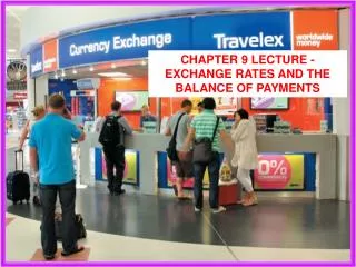
20.4 The Market for Foreign Exchange After 1971, most countries decided to abandon the fixed exchange rate system, in favor of floating exchange rates, in which the rates are determined by unregulated forces of supply and demand. Exchange rate movements have important impacts on imports, exports, and the movement of capital between countries. The Supply of and Demand for Pounds (£) Governments, private citizens, banks, and corporations exchange pounds for dollars and dollars for pounds every day. In our two-country case (U.S. and U.K.), those who demand pounds are holders of dollars seeking to exchange them for pounds. Those who supply pounds are holders of pounds seeking to exchange them for dollars.
TABLE 20.2 Some Private Buyers and Sellers in International Exchange Markets: United States and Great Britain The Demand for Pounds • Firms, households, or governments that import British goods into the United States or wish to buy British-made goods and services • U.S. citizens traveling in Great Britain • Holders of dollars who want to buy British stocks, bonds, or other financial instruments • U.S. companies that want to invest in Great Britain • Speculators who anticipate a decline in the value of the dollar relative to the pound
FIGURE 20.3 The Supply of £ in the Foreign Exchange Market When the price of £ falls, the British obtain less dollars for each pound. This means that U.S.-made goods and services appear more expensive to British buyers. A decrease in British demand for U.S. goods and services is likely to cause a fall in the quantity of £ supplied. Thus, the supply-of-pounds curve has a positive slope. FIGURE 20.2 The Demand for £ in the Foreign Exchange Market When the price of £ falls, British-made goods and services appear less expensive to U.S. buyers. If British prices are constant, U.S. buyers will buy more British goods and services and the quantity of £ demanded will rise . Hence, the demand-for-pounds curve has a negative slope.
The Equilibrium Exchange Rate FIGURE 20.4 The Equilibrium Exchange Rate When exchange rates are allowed to float, they are determined by the forces of supply and demand. An excess demand for £ will cause the price of £ to rise- the £ will appreciate with respect to the dollar (£1 will buy more dollars) . An excess supply of £ will cause the price of £ to fall- the pound will depreciate with respect to the dollar (£1 will buy less dollars). The equilibrium exchange rate occurs at the point at which the quantity demanded for £ equals the quantity of £ supplied.
20.5 Factors that Affect Exchange Rates (1) Relative Price Levels law of one price If the costs of transportation are small, the price of the same good in different countries should be roughly the same. For instance, if the price of a basketball were U$12 in the U.S. and £10 in the U.K., the exchange rate between the U.S. and the U.K. would have to be U$1.2/£. What if the exchange rate were U$1/£? (From the perspective of DD/SS of £) If would be wise to buy basketballs in the U.K. for £10, and sell them in the U.S. for U$12. This would increase the demand for £ in the U.S., thereby driving up their price to U$1.2/£.
What if the exchange rate were U$2/£? (From the perspective of DD/SS of £) It would be wise to buy basketballs in the U.S. for U$12, which costs a British about £6 per basketball. Selling them later in the U.K. at £10 would earn a profit of £4. This would increase the supply of £, and its price would fall from U$2 until it reached U$1.2. A good example of the application of the law of one price is the Big Mac Index, which looks at the prices of a Big Mac burger in Macdonald’s restaurants in about 120 different countries. If a Big Mac costs U$3 in the U.S. and £4 in the U.K., then the exchange rate would be U$0.75/£. For more details on the Big Mac Index, see http://www.economist.com/markets/bigmac/
If the law of one price held for all goods, then the purchasing power parity (PPP) is said to hold. In other words, the PPP is an aggregate application of the law of one price. The PPP asserts that if the law of one price held for all goods, and if each country consumed the same market basket of goods, the exchange rate between the two currencies would be determined simply by the relative price levels in the two countries (i.e. the ratio of the two countries’ price levels). In practice, the PPP might not hold due to significant transportation costs, insurance, storage, and/or tariffs.
FIGURE 20.5 Exchange Rates Respond to Changes in Relative Prices (from the perspective of SS and DD of £) Assume that the U.S. price level increases relative to the price level in U.K. The higher prices in the U.S. make imports relatively less expensive. U.S. citizens are likely to increase their spending on imports from U.K., shifting the demand for £ to the right, from D0 to D1. At the same time, the British see U.S. goods getting more expensive and reduce their demand for exports from the United States. The supply of £ shifts to the left, from S0 to S1. The result is an increase in the price of £. The pound appreciates against the dollar, from U$1.89 to U$2.25 per pound.
(2) Relative Interest Rates FIGURE 20.6 Exchange Rates Respond to Changes in Relative Interest Rates (from the perspective of SS and DD of £) If U.S. interest rates rise relative to British interest rates, British citizens holding £ may be attracted into the U.S. securities market. To buy bonds in the United States, British buyers must exchange £ for dollars. This implies an increase in the supply of £, shifting the supply curve to the right, from S0 to S1. However, U.S. citizens are less likely to be interested in British securities because interest rates are higher at home. The demand for £ drops and shifts to the left, from D0 to D1 (at the same time the supply of £ increases). The result is depreciation of the £ against the dollar, falling from U$1.89 to U$1.25 per pound.
20.6 The Effects of Exchange Rates on the Economy (1) Imports, Exports and Real GDP • When MYR depreciates against the dollar, the direct effects are: • a rise in the ringgit price of imports (a U$1000 machine now needs more MYR to buy); • (2) and a fall in the dollar price of Malaysian exports, though its ringgit price is fixed (a U.S. importer now needs less dollars to buy one tonne of palm oil, price at MYR3000). • The depreciation of MYR tends to bring about an increase in Malaysian exports (more competitive abroad) and a decrease in her imports (expensive imports encourage consumers to switch to domestically produced goods and services). This will cause a rise in Malaysia’s real GDP.
(2) The Balance of Trade • Balance of trade = Export Revenue – Import Costs • (BOT) = (ringgit price of exports * quantity of exports) – • (ringgit price of imports * quantity of imports) • According to the J-curve effect, when a currency starts to depreciate, the balance of trade is likely to worsen for the first few quarters. After that, it gets better. • For instance, when MYR depreciates against the dollar: • ringgit price of exports fixed; BOT unchanged • quantity of exports (not instantaneously); BOT • ringgit price of imports (instantaneously); BOT • quantity of imports (not instantaneously); BOT
FIGURE 20.7 The Effect of a Depreciation on the Balance of Trade The negative effect on the price of imports is generally felt quickly; while it takes time for export and import quantities to respond. In the short run, the value of imports increases more than the value of exports, so BOT worsens. But after exports and imports have had time to respond, the BOT turns positive.
(3) The Price Level (Inflation) • When a country’s currency depreciates, its price level will rise: • Currency depreciation increases planned AE (EX , IM), and AD curve will shift to the right. If the economy is close to capacity, the result is likely to be higher prices; • Currency depreciation makes imported inputs more expensive, shifting the AS curve to the left. If AD curve remains unchanged, the price level will increase. (4) Monetary Policy • Exchange rate is fixed: There is no role monetary policy can play. Suppose the Malaysian ringgit is fixed to USD, the central bank has no independent way of changing its interest rate. Lowering the interest rate to stimulate output will cause MYR to depreciate. • The only way to change its interest rate while keeping a fixed exchange rate is to impose capital controls (limiting the trading of MYR).
Exchange rate is flexible: • A cheaper MYR is a good thing if the goal of the expansionary monetary policyis to stimulate the domestic economy. When MS, r. A lower interest rate means a lower demand for MYR, and hence push down its value. A cheaper MYR means more exports and fewer imports, and hence Y . • Floating exchange rates also help if the central bank wants to fight inflation via contractionary monetary policy. When MS, r. The higher interest rate will push up the demand for MYR and hence its value. When MYR appreciates, the price of imports falls, shifting the AS curve to the right. If AD curve remains unchanged, the price level will drop.