Download
1 / 61
610 likes | 735 Views
AeroCom Emissions. April 2004. aerosol emission datasets. Contributors: Frank Dentener, Julian Wilson, Luisa Marelli, Jean Putaud (IES, JRC, Italy) Tami Bond (U. Washington, USA) Judith Hoelzemann, Stefan Kinne (MPI Hamburg, Germany)

E N D
AeroCom Emissions April 2004
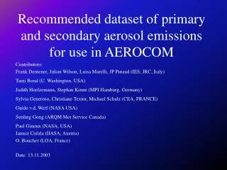
aerosol emission datasets Contributors: Frank Dentener, Julian Wilson, Luisa Marelli, Jean Putaud (IES, JRC, Italy) Tami Bond (U. Washington, USA) Judith Hoelzemann, Stefan Kinne (MPI Hamburg, Germany) Sylvia Generoso, Christiane Textor, Michael Schulz (CEA, France) Guido v.d. Werf (NASA-JPL, USA) Sunling Gong (ARQM Met Service Canada) Paul Ginoux (NOAA-GFDL, USA) Janusz Cofala (IIASA, Austria) O. Boucher (LOA, France) recommended for year 2000 simulations of AEROCOM
Goal • to provide recommended data-sets for anthropogenic aerosol and precursor gases for year 2000 simulations • including recommendations for size-distribution of primary emissions • including recommendations for emission altitude
Data-sets • Large scale biomass burning POM / EC / SO2 • Fossil fuel/biofuel related POM / BC emissions • SO2 emissions ( fossil fuel, fraction emitted as sulfate) • SEA-SALT emissions size resolved • DUST emissions size resolved • DMS (sulfur) emissions • SOA ‘effective’ emissions • Height of emissions (volcanic and biomass)
Spatial Resolution • 1 degree latitude * 1 degree longitude • averages are given for each grid-box • units are given in kg… /gridbox • for volcanic aerosol it is recommended to use the ascii-files (continuous_volc.1X1, explosive_volc.1x1) which contain the exact volcano locations NOTE: before February contained a mismatch of volcano locations
Temporal resolution • Daily emissions • DUST • SEASALT • DMS • Monthly emission • Biomass Burning • SOA • Yearly emissions • All other data-sets higher resolution data will be adopted only in sensitivity experiments
Emission Heights (1) • Dust lowest model layer < 100 m • Seasalt lowest model layer < 100 m • DMS lowest model layer < 100 m • SOA lowest model layer < 100 m • POM/BC biofuel lowest model layer < 100 m • POM/BC fossil fuel lowest model layer < 100 m • Biomass burning (OC/BC/SO2)ECO-system dependent • 0-.1km /.1-.5km /.5-1km /1-2km / 2-3km /3-6km (data provided via D. Lavoue, personal communication, 2003)
Emission Heights (2) • SO2 • domestic < 100m • road /off-road < 100m • industry 100 - 300m • shipping < 100 m • power-plants 100 - 300m • volcanic (*location and altitude are provided) • continuous 2/3 to 1/1 of volcano top * • explosive .5 to 1.5km above top *
… other data • for other data (e.g. for ‘full chemistry simulations’) it is recommended to use • EDGAR 3.2, 1995(NOx / anthropog.NMHC….)http:arch.rivm.nl/env/int/coredata/edgar • no specific recommendations are given for oxidant fields.
Data Access by anonymous ftp • ftp.ei.jrc.it … cd pub/Aerocom • subdirectories • dust_ncf • seasalt_ncf • DMS_ncf • other_ncf (or other_ascii) • BC: -biofuel, -fossil fuel, -wildfire (GFED – 6 altitude regimes) • POM: -biofuel, -fossil fue, -wildfire (GFED – 6 altitude regim.) • SO2: -domestic, -industry, -powerplants, -offroad, -road, -international shipping, -wildfire (GFED – 6 altitude regimes) • volcanic: -continuous, -explosive an overview is provided in a power-point file(Aerocom….ppt) data will be made available on CD / DVD(contact kinne@dkrz.de) File-formats: _ncf : netcdf format _ascii: ascii format _hdf: hdf format
Overview • BIOMASS BURNING • BIO FUEL / FOSSIL FUEL • SO2 • SO2 - volcanic contributions • SOA • DUST • SEASALT • DMS • EMISSION HEIGHTS • DATA ACCESS
Large scale biomass burningOC (POM) / BC (EC) / SO2 • Global emissions(incl. large agricultural fires): based on GFED 2000 REFERENCE: Van der Werf et al. : Carbon emissions from fires in tropical ecosystems, Global Change Biology, 2003 * note: in AEROCOM: we use Particulate Organic Matter (POM) rather than organic carbon (OC) - 34.7Tg POM correspond to 24.8Tg OC http://www.gps.caltech.edu/~jimr/randerson.html • compare to: • T. BondPOM34.6 Tg,OC 25.05 Tg, BC 3.32 Tg ‘open burning’ • S. GenerosoPOM 29.3 Tg,BC 3.33 Tg(ACP, 2003) • EDGAR3.2(deforestion+savannah+mid-lat.burning)SO2 2.7 Tg
size recommendationsfor primary SO4, OC and BC • particles size (log normal size-distributions) • industrial / power plant (fly ash)(larger sizes) • LN: r,mode = .500mm , std.dev = 2.0 (r,eff= 1.6mm) • biomass (based on measurement close to biomass) • LN: r,mode = .040mm , std.dev. = 1.8 (r,eff= 0.077mm) compilation by Marelli, 2003 • traffic (kerbside / urban measurements at 5 European cities) • LN: r,mode = .015 mm , std.dev. = 1.8(r,eff= 0.029 mm) based on Putaud et al. 2003 http://carbodat.ei.jrc.it/ccu/main.cfm
Young aerosol Median diameter from lognorm. Fitting (nm)
Fossil (bio-)fuel related emissionsPOM/ OC / BC • based onSPEWalso see: Tami Bond - a technology based global inventory of black and organic carbon emissions from combustion, revised to JGR, 2003. • based onGEFDfor large scale burning (open fires) note, these emissions are 35 % lower than those of a previous inventory, which was based on 1984 statistics
BC inventory comparisons • # 1 GWEM Hoelzemann • # 2 Generoso • # 3 GFED 2000 van der Werf
POM inventory comparisons • # 1 Generoso • # 2 GWEM Hoelzemann • # 3 GFED 2000 van der Werf
SO2 - emissions • Global emissions from Janusz Cofala (IIASA) Country based SO2 emissions for the year 2000 using RAINS and the EDGAR 3.2 (1995) gridded distributions (in prep.) ship - emissions: 1.5% per year increase since 1995 a flat percentage of 2.5% of all SO2 is emitted as primary SO4 (compare to 1-5% in literature)
SO2 – emissions by type decrease from 1990 to 1995 similar between EDGAR and IIASA - but IIASA+… 15 % lower than EDGAR Good correspondance with EMEP country emissions
SO2 – emissions by region / type REGIONAL ESTIMATES: kg SO2 • Region Domestic_2 Industry_2 Intern. ship Off-road_2 Powerplant RoadTransp • OPEN OCEAN 0.00e+00 0.00e+00 5.05e+09 0.00e+00 0.00e+00 0.00e+00 • CANADA 7.16e+07 1.19e+09 2.90e+07 5.30e+07 5.44e+08 1.35e+07 • USA 3.11e+08 3.12e+09 8.45e+07 1.11e+08 1.25e+10 1.67e+08 • LATIN AMERICA 1.96e+08 2.96e+09 1.71e+08 1.99e+08 2.37e+09 2.98e+08 • AFRICA 3.95e+08 1.50e+09 2.54e+08 6.90e+07 2.56e+09 1.79e+08 • OECD EUROPE 4.42e+08 2.05e+09 1.64e+09 1.89e+08 3.47e+09 1.43e+08 • EASTERN EU 6.70e+08 1.01e+09 7.73e+07 3.63e+07 4.20e+09 2.96e+07 • CIS (old UdSSR) 1.16e+09 3.99e+09 0.00e+00 1.23e+08 5.61e+09 5.82e+07 • MIDDLE EAST 5.17e+08 2.44e+09 2.32e+08 6.30e+07 2.80e+09 2.48e+08 • INDIA REGION 5.95e+08 2.90e+09 1.93e+07 1.34e+08 3.49e+09 4.36e+08 • CHINA REGION 4.76e+09 1.47e+10 1.93e+07 3.45e+08 8.73e+09 1.24e+08 • EAST ASIA 3.50e+08 2.08e+09 1.26e+08 1.55e+08 1.09e+09 1.52e+08 • OCEANIA 8.30e+06 8.06e+08 7.24e+06 4.29e+07 8.50e+08 3.67e+07 • JAPAN 6.76e+07 4.79e+08 4.10e+07 4.09e+07 2.45e+08 3.71e+07 • WORLD 9.55e+09 3.92e+10 7.75e+09 1.56e+09 4.84e+10 1.92e+09 • total world 2000: 112.5 Tg
SO2 – volcanic emissions • - continuous erupting volcanos (Andres & Kasgnoc, JGR,1998) • http://www.geiacenter.org( GEIA data [next slide] aretoo small aGEIA valuesmultiplied by factor 1.5!) • - explosive erupting volcanos • http://www.igac.noaa.gov/newsletter/22/sulfur.php
more to - volcanic emissions continuous partitioning a for more reading: • Graf et. al. : The contribution of Earth degassing to the atmospheric sulfur budget, Chem. Geology, 147, 1998. • Textor et al.: Emissions of Chemical Compounds and Aerosols in the Atmosphere, Chapter 7, 2003. • Halmer et al. : The annual volcanic gas input into the (upper) atmosphere: a global data set for the past 100 years, J. Volc. Geoth. Res., 115, 2002.
SOA - secondary organicsorganic particles from the gas phase • a fixed fraction of 15% of natural terpene emission form SOA • SOA production is more complicated • emission estim. between 10 and 60Tg/year • 19.11 Tg /year POM SOA is formed on time scales of a few hours SOA emissions condense on existing pre-existing aerosol Time resolution is 12 months
Mineral Dust • global 1*1degree daily emission data • derive emission fluxes from log-normal size-distribution parameters (fields provided in monthly netcdf-files in the “/Dust_ncf” sub-directory) • assume a dust density of 2.5g/cm3 • contributions from two size modes based on year 2000 emissions by Paul Ginoux pag@gfdl.noaa.gov Ginoux et al., JGR 102 3819-3830, 2001 Ginoux et al., Environ.M&S, 2004
Dust - Size Modes • Accumulation mode (0.1 to 1mm sizes) • Concentration /per grid-box * (mode2_number) • Mode radius (for number) (mode2_radius) • Standard deviation: 1.59 ( constant distribution width ) • Coarse mode (1 to 6 mm sizes) • Concentration /per grid-box * (mode3_number) • Mode radius (for number) (mode3_radius) • Standard deviation: 2.00 ( constant distribution width ) • conversion from “/gridbox” to “/m2” provided (gridbox_area) NOTE: for particular size-bins an idl-routine ‘binflux.pro’ (in “/help_ncf ”) is provided, which determines the emission flux (from both modes) for any given size-interval for interpolation help contact kinne@dkrz.de
Dust - yearly average mass-flux 11% of mass flux is in the accumulation mode (acc) 89% of the mass flux is in the coarse mode (coa) 70% more than IPCC-TAR
Sea-Salt • global 1*1degree daily emission data • derive emission fluxes from log-normal size-distribution parameters (fields provided in monthly netcdf-files in the “/seasalt_ncf” sub-directory) • assume a dry sea-salt density of 2.2g/cm3 • contributions from three size modes based on year 2000 emissions by Sunling.Gong@ec.gc.ca (here only sizes smaller than 20mm diameter are considered) Gong et.al. JGR, 107, 2002, Gong and Barrie, JGR, 108, 2003, Gong Glo.Bio.Cycles, 17, 2003
Sea-Salt Size Modes • Aitken mode (sizes smaller than 0.1mm) • Concentration /per grid-box * (mode1_number) • Mode radius (for number) (mode1_radius) • Standard deviation: 1.59 (distribution width) • Accumulation mode (0.1 to 1mm sizes) • Concentration /per grid-box * (mode2_number) • Mode radius (for number) (mode2_radius) • Standard deviation: 1.59 (distribution width) • Coarse mode (1 to 20 mm sizes) • Concentration /per grid-box * (mode3_number) • Mode radius (for number) (mode3_radius) • Standard deviation: 2.00 (distribution width) “/gridbox” to “/m2” conversion data provided ‘binflux.pro’ calculates fluxes for any size bin(“/help_ncf”)