Download
1 / 37
370 likes | 486 Views
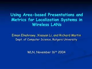
Using Area-based Presentations and Metrics for Localization Systems in Wireless LANs. E. Elnahrawy, X. Li, and R. Martin Rutgers U. WLAN-Based Localization. Localization in indoor environments using 802.11 and Fingerprinting Numerous useful applications

E N D
Using Area-based Presentations and Metrics for Localization Systems in Wireless LANs E. Elnahrawy, X. Li, and R. Martin Rutgers U.
WLAN-Based Localization • Localization in indoor environments using 802.11 and Fingerprinting • Numerous useful applications • Dual use infrastructure: a huge advantage
[(x,y),s1,s2,s3] [(x,y),s1,s2,s3] [(x,y),s1,s2,s3] Background: Fingerprinting Localization • Classifiers/matching/learning approaches • Offline phase: • Collect training data (fingerprints) • Fingerprint vectors: [(x,y),SS] • Online phase: • Match RSS to existing fingerprints probabilistically or using a distance metric RSS [-80,-67,-50] (x?,y?)
Background (cont) • Output: • A single location: the closest/best match • We call such approaches “Point-based Localization” • Examples: • RADAR • Probabilistic approaches [Bahl00, Ladd02, Roos02, Smailagic02, Youssef03, Krishnan04]
Contributions: Area-based Localization • Returned answer is area/volume likely to contain the localized object • Area is described by a set of tiles • Ability to describe uncertainty • Set of highly possible locations
Contributions: Area-based Localization • Show that it has critical advantages over point-based localization • Introduce new performance metrics • Present two novel algorithms: SPM and ABP-c • Evaluate our algorithms and compare them against traditional point-based approaches • Related Work: different technologies/algorithms [Want92, Priyantha00, Doherty01, Niculescue01, Savvides01, Shang03, He03, Hazas03, Lorincz04]
Why Area-based? • Noise and systematic errors introduce position uncertainty • Areas improve system’s ability to givemeaningful alternatives • A tool for understanding the confidence • Ability to trade Precision(area size) for Accuracy(distance the localized object is from the area) • Direct users in their search • Yields higher overall accuracy • Previous approaches that attempted to use areas only use them as intermediate result output still a single location
Area-based vs. Single-Location 80 • Object can be in a single room or multiple rooms • Point-based to areas • Enclosing circles -- much larger • Rectangle? no longer point-based! 70 60 50 40 30 20 10 0 0 200 0 200
Outline • Introduction, Motivations, and Related Work • Area-based vs. Point-based localization • Metrics • Localization Algorithms • Simple Point Matching (SPM) • Area-based Probability (ABP-c) • Interpolated Map Grid (IMG) • Experimental Evaluation • Conclusion, Ongoing and Future Work
Performance Metrics • Traditional: Distance error between returned and true position • Return avg, 95th percentile, or full CDF • Does not apply to area-based algorithms! • Does not show accuracy-precision tradeoffs!
New Metrics: Accuracy Vs. Precision • Tile Accuracy % true tile is returned • Distance Accuracy distance between true tile and returned tiles (sort and use percentiles to capture distribution) • Precision size of returned area (e.g., sq.ft.) or % floor size
Room-Level Metrics • Applications usually operate at the level of rooms • Mapping: divide floor into rooms and map tiles • (Point -> Room): easy • (Area -> Room): tricky • Metrics: accuracy-precision • Room Accuracy % true room is the returned room • Top-n rooms Accuracy % true room is among the returned rooms • Room Precision avg number of returned rooms
∩ ∩ = 1. Simple Point Matching (SPM) • Build a regular grid of tiles, match expected fingerprints • Find all tiles which fall within a “threshold” of RSS for each AP • Eager: start from low threshold (s, 2s, 3s , …) • Threshold is picked based on the standard deviation of the received signal • Similar to Maximum Likelihood Estimation
2. Area-Based Probability (ABP-c) Build a regular grid of tiles, tile ↔ expected fingerprint Using “Bayes’ rule” compute likelihood of an RSS matching the fingerprint for each tile p(Ti|RSS) α p(RSS|Ti) . p(Ti) Return top tiles bounded by an overall probability that the object lies in the area (Confidence: user-defined) Confidence ↑ → Area size ↑
90 85 80 75 70 65 60 140 55 50 45 40 y in feet 0 210 x in feet Measurement At Each Tile Is Expensive! • Interpolated Map Grid: (Surface Fitting) • Goal: Extends original training data to cover the entire floor by deriving an expected fingerprint in each tile • Triangle-based linear interpolation using “Delaunay Triangulation” • Advantages: • Simple, fast, and efficient • Insensitive to the tile size
Impact of Training on IMG • Both location and number of training samples impact accuracy of the map, and localization performance • Number of samples has an impact, but not strong! • Little difference going from 30-115, no difference using > 115 training samples • Different strategies [Fixed spacing vs. Average spacing]: as long as samples are “uniformly distributed” but not necessarily “uniformly spaced” methodology has no measurable effect
Experimental Setup • CoRE • 802.11 data: 286 fingerprints (rooms + hallways) • 50 rooms • 200x80 feet • 4 Access Points
Average Overall Room Accuracy Average Overall Precision 100 10 SPM ABP-50 95 ABP-75 8 ABP-95 90 85 6 % accuracy 80 % floor 4 75 SPM 70 ABP-50 2 ABP-75 65 ABP-95 60 0 0 50 100 150 200 250 0 50 100 150 200 250 Training data size Training data size Area-based Approaches: Accuracy-Precision Tradeoffs • Improving Accuracy worsens Precision(tradeoff)
ABP-50: Percentiles' CDF ABP-75: Percentiles' CDF 1 1 0.8 0.8 probability probability 0.6 0.6 0.4 0.4 Minimum Minimum 25 Percentile 25 Percentile 0.2 0.2 Median Median 75 Percentile 75 Percentile Maximum Maximum 0 0 0 20 40 60 80 100 0 20 40 60 80 100 ABP-95: Percentiles' CDF 1 0.8 0.6 probability 0.4 Minimum 25 Percentile 0.2 Median 75 Percentile Maximum 0 0 20 40 60 80 100 distance in feet A Deeper Look Into “Accuracy” SPM: Percentiles' CDF 1 0.8 0.6 probability 0.4 Minimum 25 Percentile 0.2 Median 75 Percentile Maximum 0 0 20 40 60 80 100 distance in feet
ABP-50 ABP-75 SPM ABP-95 Sample Outputs • Area expands into the true room • Areas illustrate bias across different dimensions (APs’ location)
Comparison With Point-based localization: Evaluated Algorithms • RADAR • Return the “closest” fingerprint to the RSS in the training set using “Euclidean Distance in signal space” (R1) • Averaged RADAR (R2), Gridded RADAR (GR) • Highest Probability • Similar to ABP: a typical approach that uses “Bayes’ rule” but returns the “highest probability single location” (P1) • Averaged Highest Probability (P2), Gridded Highest Probability (GP)
Comparison With Point-based Localization: Performance Metrics • Traditional error along with percentiles CDF for area-based algorithms (min, median, max) • Room-level accuracy
Min Median Max CDFs for point-based algorithms fall in-between the min, max CDFs for area-based algorithms Point-based algorithms perform more or less the same, closely matching the median CDF of area-based algorithms
Similar top-room accuracy Area-based algorithms are superior at returning multiple rooms, yielding higher overall room accuracy If the true room is missed in point-based algorithms the user has no clue!
Conclusion • Area-based algorithms present users a more intuitive way to reason about localization uncertainty • Novel area-based algorithms and performance metrics • Evaluations showed that qualitatively all the algorithms are quite similar in terms of their accuracy • Area-based approaches however direct users in their search for the object by returning an ordered set of likely rooms and illustrate confidence
System for LEASE: Location Estimation Assisted by Stationary Emitters for Indoor RF wireless Networks P. Krishnan, A.S. Krishnakumar, W.H. Ju, C. Mallows, S. Ganu Avaya Labs and Rutgers
LEASE components • Access Points • Normal 802.11 access points • Stationary Emitters • Emit packets, placed throughout floor • Sniffers • Read packets sent by AP, report signal strength fingerprint • Location Estimation Engine (LEE) • Server to compute the locations
LEASE methodology • SE emit packets • Sniffers report fingerprints to LEE • LEE builds a radio map via interpolation • Divide floor into a grid of tiles • Estimate RSS of each SE for each tile • Result is an estimated fingerprint for each tile • Client sends packet • Sniffers measure RSS of client packet • LEE computes location of client based on the map.
Building the map • For a each sniffer: • have X, Y, RSS (“height”) for each AP • Use a generalized adaptive model to smooth the data. • Use Akima splines to build an interpolated “surface” from the set of “heights” over the grid of tiles • Each tile(3ftx3ft) has a predicted RSS for the sniffer • Note complexity vs. the Delaunay triangles for SPM, APB algorithms.
Matching the Clients • Sniffers receive RSS of a client packet • Find the tile with the closest matching set of RSSs • Compute the distance in “signal space” • Sqrt( (RSS-RSS) ^2 + (RSS-RSS) … • Full-NNS: match the entire vector for each RSS • Top-K: match only the strongest K-signals
Metric • Want to combine several factors into a single numeric value to judge the localization system • Factors: • Area covered (A) • (more -> better) • # of fingerprints (k) • (more -> worse) • Localization error (m) • (more -> worse)
Metric (lower is better) # of fingerprints Relative weights Scaling Constant Median error Area of location system
Using the Metric Note, areas for first 2 are normalized to the Corridors (whole floor doesn’t count)
Questions: • What are meaningful numbers? • What to count in A? • Corridor only? • What happens to m vs A? • E.g. if we measure only in the corridors, but then try to localize in the rooms? • What should the weights be?