Download
1 / 17
170 likes | 282 Views
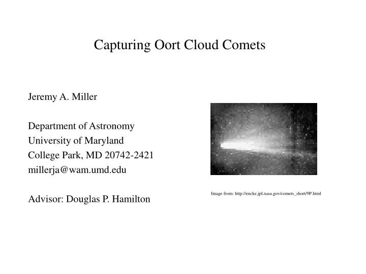
Capturing Oort Cloud Comets. Jeremy A. Miller Department of Astronomy University of Maryland College Park, MD 20742-2421 millerja@wam.umd.edu Advisor: Douglas P. Hamilton. Image from: http://encke.jpl.nasa.gov/comets_short/9P.html. An introduction to comets.

E N D
Capturing Oort Cloud Comets Jeremy A. Miller Department of Astronomy University of Maryland College Park, MD 20742-2421 millerja@wam.umd.edu Advisor: Douglas P. Hamilton Image from: http://encke.jpl.nasa.gov/comets_short/9P.html
An introduction to comets • Halley – comets orbit the Sun periodically. • Oort – comets come from a spherical shell ~20,000 AU away. • Kuiper – other comets come from a flat ring 30-50AU away. Image from: http://dsmama.obspm.fr/demo/comet.gif
Numerical methods • Everhart 1969 (E69): • Patched conic method around Jupiter • Single passes by same comet • Everhart 1972 (E72): • Numerical integration with Jupiter and Sun • Multiple passes by same comet • Wiegert and Tremaine 1999 (WT): • N-body simulation with all planets and Sun • Multiple passes by same comet Image from: http://science.howstuffworks.com/planet-hunting1.htm
Why simplify the problem? N-body simulations may give more accurate results than analytic methods... But analytic methods and impulse approximations are easier to understand physically. Image from: http://www.lactamme.polytechnique.fr/Mosaic/images/NCOR.C3.0512.D/display.html
Two coordinate systems The Jupiter-comet system: *Jupiter bends a comet’s orbit. *Jupiter can give or take energy. *Sun’s influence on comet ignored. The Sun-comet system: *Comet follows Keplerian orbit around sun. *Orbital elements used to describe motion. *Jupiter’s influence on comet ignored. We approximate the motion of Oort cloud comets by combining these two systems.
The Jupiter-comet system • Comets spending more time in front of Jupiter than behind are captured. • The magnitude of the comet’s deflection depends on its speed relative to Jupiter and the distance of closest approach. • Fast comets barely deflected • Slow comets deflected quite a bit Image from: http://analyzer.depaul.edu/paperplate/PPE%20pause/Dynamic%20comet.jpg
The Sun-comet system:Tisserand’s Criterion *Valid for single planet on a circular orbit *Valid when comet is far from Jupiter *Combination of energy and angular momentum
The Sun-comet system:Special case • io = 90o pericenter encounter • K=0 • increased inclination = capture • decreased inclination = escape • exactly one circular orbit General case • Bound orbits have smaller final than initial z angular momentum • Retrograde comets cannot produce prograde elliptical orbits
Three-body impulse approximation algorithm Sun-comet coordinate system Jupiter-comet coordinate system (The “target plane”) The parameters b, g, r and q uniquely define an interaction (b, g) – Angles that define the comet’s velocity (r, q) – Position of closest approach on the target plane Image from: http://nmp.jpl.nasa.gov/ds1/edu/comets.html
The algorithm (sans gory details) 0) Start with parabolic orbit comets velocity v = √2 1) Choose geometry parameters b, g, r, and q. 2) Convert to velocity vectors. 3) Impulse: rotate velocity vector by a in Jupiter-comet coordinate system. 4) Convert final velocity into final parameters. 5) Convert final parameters to heliocentric orbital elements. Just solve this equation... simple!
Monte Carlo approach:Repeat steps 500 million times (We used a computer for this part) We assumed a spherically symmetric distribution of massless comets on parabolic orbits: b, g , x=rcosq, and y=rsinq chosen randomly rmax chosen to be 200rj. Image from: http://www.educeth.ch/stromboli/photoastro/index-en.html
Results *<a> > 0 (51.4% of comets captured) *<i> > 90o (51.0% of comets retrograde) -but- Problem: Tisserand’s constant should be conserved. We find it increases by ~1%. Lets look at some orbital element distributions... Image from: http://www2.jpl.nasa.gov/sl9/gif/kitt11.gif
More results for captured comets Comets highly elliptical – weak interactions Most semimajor axes less than 20 aj Retrograde orbits – Tisserand’s criterion Low inclination peak – geometry Pericenter distribution unchanged
SPCs, HTCs, and LPCs SPCs are more strongly peaked at lower inclinations than HTCs Why? Geometry SPCs have a larger spread of eccentricities than LPCs Why? Stronger interactions
Future work Our main goal is to find and explain trends in cometary distributions using simple physics. To further this goal we will: *Track down error in K *Compare results to numerical integrations *Run multiple passes of comets by Jupiter *Make more graphs for more insight Image from: http://flaming-shadows.tripod.com/gal2.htm
Acknowledgements I want to thank my advisor, Doug Hamilton, for all of his help on this project. I couldn’t have done it without him (or gotten away with using the royal “we”) . I also want to thank the astronomy department for the use of their computer labs. These people helped a bit as well: Quote from: http://www.wilsonsalmanac.com/constantinople.html