Analytical solutions of 2 1 dimensional Burgers equation with damping term by HPM,ADM and DTM

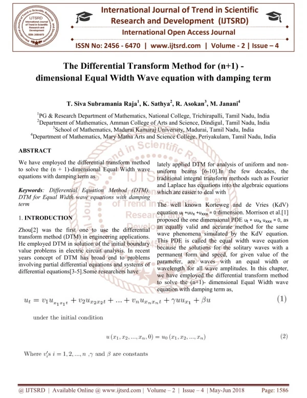
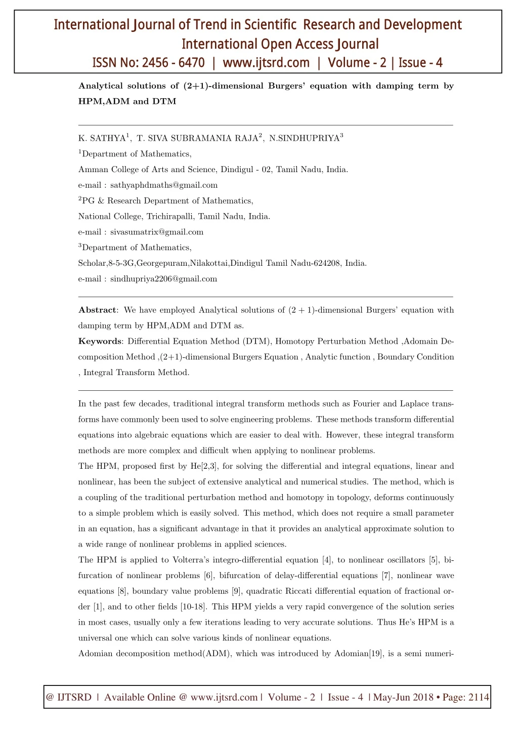
1. International Journal of Trend in Scientific Research and Development International Open Access Journal ISSN No: 2456 - 6470 | www.ijtsrd.com | Volume - 2 | Issue - 4 Analytical solutions of (2+1)-dimensional Burgers’ equation with damping term by HPM,ADM and DTM K. SATHYA1, T. SIVA SUBRAMANIA RAJA2, N.SINDHUPRIYA3 1Department of Mathematics, Amman College of Arts and Science, Dindigul - 02, Tamil Nadu, India. e-mail : sathyaphdmaths@gmail.com 2PG & Research Department of Mathematics, National College, Trichirapalli, Tamil Nadu, India. e-mail : sivasumatrix@gmail.com 3Department of Mathematics, Scholar,8-5-3G,Georgepuram,Nilakottai,Dindigul Tamil Nadu-624208, India. e-mail : sindhupriya2206@gmail.com Abstract: We have employed Analytical solutions of (2 + 1)-dimensional Burgers’ equation with damping term by HPM,ADM and DTM as. Keywords: Differential Equation Method (DTM), Homotopy Perturbation Method ,Adomain De- composition Method ,(2+1)-dimensional Burgers Equation , Analytic function , Boundary Condition , Integral Transform Method. In the past few decades, traditional integral transform methods such as Fourier and Laplace trans- forms have commonly been used to solve engineering problems. These methods transform differential equations into algebraic equations which are easier to deal with. However, these integral transform methods are more complex and difficult when applying to nonlinear problems. The HPM, proposed first by He[2,3], for solving the differential and integral equations, linear and nonlinear, has been the subject of extensive analytical and numerical studies. The method, which is a coupling of the traditional perturbation method and homotopy in topology, deforms continuously to a simple problem which is easily solved. This method, which does not require a small parameter in an equation, has a significant advantage in that it provides an analytical approximate solution to a wide range of nonlinear problems in applied sciences. The HPM is applied to Volterra’s integro-differential equation [4], to nonlinear oscillators [5], bi- furcation of nonlinear problems [6], bifurcation of delay-differential equations [7], nonlinear wave equations [8], boundary value problems [9], quadratic Riccati differential equation of fractional or- der [1], and to other fields [10-18]. This HPM yields a very rapid convergence of the solution series in most cases, usually only a few iterations leading to very accurate solutions. Thus He’s HPM is a universal one which can solve various kinds of nonlinear equations. Adomian decomposition method(ADM), which was introduced by Adomian[19], is a semi numeri- 1 @ IJTSRD | Available Online @ www.ijtsrd.com | Volume - 2 | Issue - 4 | May-Jun 2018 • Page: 2114

2. International Journal of Trend in Scientific Research and Development (IJTSRD) ISSN: 2456-6470 cal technique for solving linear and nonlinear differential equations by generating a funtional series solution in a very efficient manner. The method has many advantages: it solves the problem di- rectly without the need for linearization, perturbation, or any other transformation; it converges very rapidly and is highly accurate. Differential transform method (DTM),which was first applied in the engineering field by Zhou[8],has many advantages :it solves the problem directly without the need for linearization,pertuburation,or any other transformation.DTM is based on the Taylors series expansion.It is different from the tradi- tional high order Taylor series method,which needs symbolic computation of the necessary derivatives of the data functions.Taylor series method computationally takes a long time for larger orders while DTM method reduces the size of the computational domain,without massive computations and re- strictive assumpions,and is easily applicable to various physical problems .The method and related theorems are well adressed in [9,10].Let us consider the (2+1)-dimensional Burgers’ equation with damping term as, (1) ut= uxuy+ u + uxy, under the initial condition (2) u(x,y,0) = u0(x,y). Burger’s equation is the simplest second order NLPDE which balances the effect of nonlinear convection and the linear diffusion.In this work ,we have employed the Homotopy Perturbation Method(HPM),DTM and ADM to solve the (2+1)dimensional Burger’s equation with damping term. 1.1 Homotopy Perturbation Method (HPM) To describe the HPM, consider the following general nonlinear differential equation (3) A(u) − f(r) = 0,r?Ω, under the boundary condition B(u,∂u (4) ∂n) = 0,r?∂Ω, Where A is a general differential operator, B is a boundary operator,f(r)is a known analytic function and ∂Ω is a boundary of the domain Ω.The operator A can be divided into two parts L and N, Where L is a linear opertor while N is a nonlinear operator.Then Equation(3)can be rewritten as (5) L(u) + N(u) − f(r) = 0, Using the homotopy tecnique, we construct a homotopy: V (r,p) : ΩX[0,1] → R 2 @ IJTSRD | Available Online @ www.ijtsrd.com | Volume - 2 | Issue - 4 | May-Jun 2018 • Page: 276 @ IJTSRD | Available Online @ www.ijtsrd.com | Volume - 2 | Issue - 4 | May-Jun 2018 • Page: 276 @ IJTSRD | Available Online @ www.ijtsrd.com | Volume - 2 | Issue - 4 | May-Jun 2018 • Page: 2115

3. International Journal of Trend in Scientific Research and Development (IJTSRD) ISSN: 2456-6470 Which satisfies H(V,p) = (1 − p)[L(V ) − L(u0)] + p[A(V ) − f(r)] or (6) H(V,p) = L(V ) − L(u0) + pL(u0) + p[N(V ) − f(r)],r?Ω,p?[0,1], Where p?[0,1] is an embedding parameter, u0 is the initial approximation of Equation(3) which satisfies the boundary conditions.Obviously,considering Equation(6),we will have H(V,0) = L(V ) − L(u0) = 0, (7) H(V,1) = A(V ) − f(r) = 0, changing the process of p from zero to unity is just that V(r,p)from u0(r) to u(r).In topology,this is called the deformation also A(V)-f(r) and L(u)are called as homotopy .The homotopy perturbation method uses the homotopy parameter p as an expanding parameter [23-25]to obtain ∞ X V = v0+ pv1+ p2v2+ p3v3+ ... = pnvn. (8) n=0 p →1 results the appropriate solution of equation(3)as ∞ X u = lim p→1V = v0+ v1+ v2+ ... = vn. (9) n=0 A comparision of like powers of p gives the solutions of various orders series(9)is convergent for most of the cases.However convergence rate depends on the nonlinear,N(V ) He[25]suggested the following opinions: 1.The second derivative of N(V)with respect to v must be small as the parameter p may be relatively large. 2.The norm of L−1∂N must be smaller than one so that the series converges. In this section, we ∂u describe the above method by the following example to validate the efficiency of the HPM. Example:1 Consider the (2+1)-dimensional Burgers’ equation with daming as, (10) ut= uxy+ uxuy+ u, under the initial condition (11) u(x,y,0) = u0(x,y) = x + y. Applying the homotopy perturbation method to Equation(10),we have (12) ut+ p[(−uxy− uux− u)] = 0. 3 @ IJTSRD | Available Online @ www.ijtsrd.com | Volume - 2 | Issue - 4 | May-Jun 2018 • Page: 2116

4. International Journal of Trend in Scientific Research and Development (IJTSRD) ISSN: 2456-6470 In the view of HPM, we use the homotopy parameter p to expand the solution u(x,y,t) = u0+ pu1+ p2u2+ ... (13) The approximate solution can be obtained by taking p=1 in equation (13)as (14) u(x,y,t) = u0+ u1+ u2+ ... Now substituing equation(12)into equation(11)and equating the terms with identical powers of p, we obtain the series of linear equations, which can be easily solved.First few linear equations are given as p0:∂u0 (15) = 0 ∂t =∂2u0 p1:∂u1 ∂x∂y+∂u0 ∂u0 ∂y (16) + u0. ∂t ∂x =∂2u1 p2:∂u2 ∂x∂y+∂u1 ∂u0 ∂y +∂u0 ∂u1 ∂y (17) + u1. ∂t ∂x ∂x Using the initial condition(11), the soution of Equation(15)is given by (18) u(x,y,0) = u0(x,y) = (x + y). Then the solution of Equation(16)will be ?∂2u0 ? t Z o ∂x∂y+∂u0 ∂u0 ∂y (19) u1(x,y,t) = + u0 dt. ∂x (20) u1(x,y,t) = (x + y)t + t. Also, We can find the solution of Equation(17)by using the following formula ?∂2u1 ? t Z 0 ∂x∂y+∂u1 ∂u0 ∂y +∂u0 ∂u1 ∂y (21) u1(x,y,t) = + u1 dt. ∂x ∂x u2(x,y,t) = (x + y)t2 2!+3t2 (22) 2! etc.therefore, from equation(18),the approximate solution of equation(10)is given as u(x,y,t) = (x + y) + (x + y)t + t +t2 2!+3t2 (23) + ... 2! Hence the exact solution can be expressed as u(x,y,t) = (x + y)et+ (n! + 1)(et− 1), (24) provided that 0 ≤ t < 1 4 @ IJTSRD | Available Online @ www.ijtsrd.com | Volume - 2 | Issue - 4 | May-Jun 2018 • Page: 2117

5. International Journal of Trend in Scientific Research and Development (IJTSRD) ISSN: 2456-6470 1.2 Adomain Decomposition Method(ADM) Consider the following linear operatpor and their inverse operators: ∂2 Lt=∂ ∂t;Lx,y= ∂x∂y. y t Z 0 Z 0 Z 0 x L−1 t = (.)dt,Lx,y= (.)dτdγ. Using the above notations,Equation(1)becomes (25) Lt(u) = Lx,y(u) + uxuy, Operating the inverse operators L−1 to equation(25)and using the initial condition gives t u(x,y,t) = u0(x,y,t) + L−1 t (Lx,y(u)) + L−1 (26) t (uxuy), The decomposition method consists of representing the solution u(x,y,t)by the decomposition series ∞ X u(x,y,t) = uq(x,y,t). (27) q=0 The nonlinear term uxuyis represented by a series of the so called Adomain polynomials, given by ∞ X u = Aq(x,y,t). (28) q=0 The component uq(x,y,t) of the solution u(x,y,t)is determined in a recursive manner.Replacing the decomposition series (27)and(26)gives ∞ X ∞ X uq(x,y,t) = u0(x,y,t) + L−1 t (Lx,y,t(u)) + L−1 Aq(x,y,t) (29) t q=0 q=0 According to ADM the zero-th component u0(x,y,t) is identified from the initial or boundary cndi- tions and from the source terms.The remaining components of u(x,y,t) are determined in a recursion manner as follows (30) u0(x,y,t) = u0(x,y), uk(x,y,t) = L−1 t (Lx,y(u)) + L−1 (31) t (Ak),k ≥ 0, Where thhe adomain polynomials for the nonlinear term uxuyare derived from the following recursive formulation ∞ ! ∞ !! X X dk dλk Ak=1 λiui λiui ,k = 0,1,2,... (32) k! i=0 i=0 λ=0 First few Adomian polynomials are given as A0= u0∂u0 ∂x1,A1= u0∂u1 + u1∂u0 ∂x1, ∂x1 5 @ IJTSRD | Available Online @ www.ijtsrd.com | Volume - 2 | Issue - 4 | May-Jun 2018 • Page: 2118

6. @ IJTSRD | Available Online @ www.ijtsrd.com | Volume - 2 | Issue - 4 | May-Jun 2018 • Page: 276 International Journal of Trend in Scientific Research and Development (IJTSRD) ISSN: 2456-6470 A2= u2∂u0 + u1∂u1 + u0∂u2 (33) ∂x1, ∂x1 ∂x1 using equation(31)for the adomain polynomials Ak,we get (34) u0(x,y,t) = u0(x,y), u1(x,y,t) = L−1 t (Lx,y(u0)) + L−1 (35) t (A0), u2(x,y,t) = L−1 t (Lx,y(u1)) + L−1 (36) t (A1), and so on.Then the q-th term, uqcan be determined from q−1 X (37) uq= uk(x,y,t). 0 Knowing the components of u, the analytical solution follows immediately. 1.2.1 Computational illustrations of ADM for (n+1)-dimensional Burgers’ equation with damping using Equations(32) and (33), first few components of the decomposition series are given by (38) u0(x,y,t) = (x + y), (39) u1(x,y,t) = (x + y)t + t, u2(x,y,t) = (x + y)t2 2!+3t2 3!+7t3 (40) 2!, u3(x,y,t) = (x + y)t3 (41) 3!, ∞ X u(x,y,t) = uk(x,y,t) k=0 = u0(x,y,t) + u1(x,y,t) + u2(x,y,t) + ..., = (x + y) + (x + y)t + t +3t2 + (x + y)t2 2!+ (x + y)t3 3!+7t3 (42) + ... 2! 3! Hence, the exact solution can be expressed as u(x,y,t) = (x + y)et+ (n! + 1)(et− 1) (43) 1.3 Differential Transform Method(DTM) In this section,we give some basic definitions of the differential transformation.Let D denotes the differential transform operator and D−1the inverse differential transform operator. 6 @ IJTSRD | Available Online @ www.ijtsrd.com | Volume - 2 | Issue - 4 | May-Jun 2018 • Page: 2119

7. International Journal of Trend in Scientific Research and Development (IJTSRD) ISSN: 2456-6470 1.3.1 Basic Definition of DTM Definition:1 If u(x1,x2,...,xn,t) is analytic in the domain Ω then its (n+1)- dimensional differential transform is given by ? ? 1 × U (k1,k2,...,kn,kn+1) = k1!,k2!,...,kn!,kn+1! ∂k1+k2+...+kn+kn+1 ∂k1 (44) .u(x1,x2,...,xn,t)|x1= 0,x2= 0,...,xn= 0,t = 0 xn∂kn+1 xt x1∂k2 x2...∂kn where ∞ X ∞ X ∞ X ∞ X U (k1,k2,...,kn,kn+1).xk1 1xk2 2...xkn ntkn+1 u(x1,x2,...,xn,t) = ... (45) k1=0 k2=0 kn=0 kn+1=0 = D−1[U (k1,k2,...,kn,kn+1)] Definition:2 If u(x1,x2,...,xn,t) = D−1[u(k1,k2,...,kn,kn+1)],v(x1,x2,...,xn,t) = D−1[V (k1,k2,...,kn,kn+1)],and ⊗ denotes convolution,then the fundamental operations of the differential transform are expressed as follows: (a).D[u(x1,x2,...,xn,t)v(x1,x2,...,xn,t)] = U(k1,k2,...,kn,kn+1) ⊗ V (k1,k2,...,kn,kn+1) k1 X kn+1 X (46) k2 X kn X U(a1,k2− a2,...,kn+1− an+1)V (k1− a1,a2,...,an+1) = ... a1=0 a2=0 an=0 an+1=0 (47) (b).D[αu(x1,x2,...,xn,t) ± βv(x1,x2,...,xn,t)] = αU(k1,k2,...,kn,kn+1) (c).D∂k1+k2+...+kn+kn+1 ∂k1 xt .u(x1,x2,...,xn,t) = (k1+ 1)(k1+ 2)...(k1+ r1)(k2+ 1)(k2+ 2) xn∂kn+1 x1∂k2 x2...∂kn (48) ...(k2+ r2)...(kn+1+ 1)(kn+1+ 2)...(kn+1+ rn+1).U(k1+ r1,...,kn+1+ rn+1) 1.3.2 Computational illustrations of (2+1)-dimensional Burgers’ equation with damping Here we describe the method explained in the previous section, by the following to validate the efficiency of the DTM Consider the (2+1)-dimensional Burgers’ equation with damping as, (49) ut= uxy+ uxuy+ u, Subject to the initial condition (50) u(x,y,0) = u0(x,y) = x + y Talking the differential transform of equation(49).,we have (k3+ 1)U(k1,k2,k3+ 1) = (k1+ 2)(k1+ 1)U(k1+ 1,k2+ 1,k3) + U(k1,k2,k3) (51) +U(a1,k2− a2,k3− a3) + U(k1− a1,a2,k3− a3) 7 @ IJTSRD | Available Online @ www.ijtsrd.com | Volume - 2 | Issue - 4 | May-Jun 2018 • Page: 2120

8. International Journal of Trend in Scientific Research and Development (IJTSRD) ISSN: 2456-6470 From the initial condition equation(50),it can beseen that ∞ X ∞ X U(k1,k2,0)(xk1.yk2) = x + y u(x,y,0) = (52) k1=0 k2=0 Where       1  if ki= 1,kj= 0, i 6= j,i,j=1,2 otherwise 1 U(k1,k2,0) = (53) 0 Using eq.(53)into eq.(52)one can obtain the values of U(k1,k2,k3,k4) as follows    if ki= 1,kj= 0, i 6= j,i,j=1,2 otherwise 1 U(k1,k2,1) = (54) 0      if ki= 1, kj= 0,i 6= j, i, j = 1,2 otherwise U(k1,k2,2) = (55) 0 Then from eqn.(45)we have ∞ X ∞ X U(k1,k2,k3)xk1yk2tk3 u(x,y,t) = k1=0 k2=0 = (x + y) + (x + y)t + t +3t2 + (x + y)t2 2!+ (x + y)t3 3!+7t3 (56) + ... 2! 3! Hence,the exact solution is given by u(x,y,t) = (x + y)et+ (n! + 1)(et− 1) (57) 1.4 Conclusion 1.In this work,homotopy perturbation methhod,DTM and adomian decomposition method have been successfully applied for solving (2+1)-dimensional Burgers’ equation with damping term. 2.The solutions obtained by these methods are an infinite power series for an appropriate initial condition, which can,in turn be expressed in a closed form, the exact solution. 3.The results reveal that the methods are very effective, convenient and quite accurate mathe- matical tools for solving the (2+1)-dimensional Burgers’ equation equation with damping. 4.The solution is calculated in the form of the convergent power series with easily computable components. 5.These method, which can be used without any need to complex computations. 1.5 References [1].Z.Odibat,S.Momani, Chaos Solitons Fractals,in press. [2]. J.H.He, Comput. Methods Appl.Mech. Engrg. 178,(1999),257. 8 @ IJTSRD | Available Online @ www.ijtsrd.com | Volume - 2 | Issue - 4 | May-Jun 2018 • Page: 2121

9. International Journal of Trend in Scientific Research and Development (IJTSRD) ISSN: 2456-6470 [3]. J.H.He,Int.J.Non-linear Mech., 35(1),(2000),37 [4]. M.El-Shahed, Int.J.Nonlin.sci. Numer. Simul., 6(2),(2005),163. [5]. J.H.He, Appl. Math. Comput.,151,(2004),287 [6]. J.H.He,Int.J.Nonlin.Sci.Numer.Simul.,6(2),(2005),207 [7]. J.H.He, Phys. Lett. A ,374,(4-6),(2005),228. [8]. J.H.He,Chaos Solitons Fractals,26(3),(2005),695. [9]. J.H.He,Phys.Lett.A,350,(1-2),(2006),87. [10]. J.H.He, Appl. Math. Comput.,151,(2003),73 [11]. J.H.He,Appl.Math.Comput.,156,(2004),527. [12]. J.H.He,Appl.Math.Comput.,156,(2004),591. [13]. J.H.He, Chaos Solitons Fractals,26,(3),(2005),827. [14]. A.Siddiqui, R.Mahmood, Q.Ghori, Int. J.Nonlin. Sci. Numer. Simul.,7(1),(2006),7. [15]. A.Siddiqui, R.Ahmed, Q.Ghori, Int. J.Nonlin. Sci. Numer. Simul.,7(1),(2006),15. [16]. J.H.He,Int.J.Mod. Phys.B,20,(10),(2006),1141. [17]. S.Abbasbandy,Appl.Math.Comput.,172,(2006),485. [18]. S.Abbasbandy,Appl.Math.Comput.,173,(2006),493. [19]. G.Adomain. A review of the decomposition method in applied mathematics., J Math Anal Appl,(1988),135,501-544. [20]. F.J.Alexander, J.L.Lebowitz. Driven diffusive systems with a moving obstacle variation on the Brazil nuts problem.J Phys(1990),23,375-382. [21]. F.J.Alexander, J.L.Lebowitz., On the drift and diffusion of a rod in a lattice fluid. J Phys(1994),27,683-696. [22]. J.D.Cole., On a quasilinear parabolic equation occurring in aerodynamics. J Math Appl, (1988),135,501-544. [23]. He JH.Homotopy perturbation technique.Comput methods Appl Mech Eng, (1999),178,257-262. [24]. J.H.He., Homotopy perturbation method: a new nonlinear analytical technique., Appl Math Comput,(2003),13,(2-3), 73-79. [25] J.H. He.,A simple perturbation method to Blasius equation. Appl Math Comput, (2003),(2-3),217-222. 9 @ IJTSRD | Available Online @ www.ijtsrd.com | Volume - 2 | Issue - 4 | May-Jun 2018 • Page: 2122