Data Layout Transformation for Enhancing Data Locality on NUCA Chip Multiprocessors

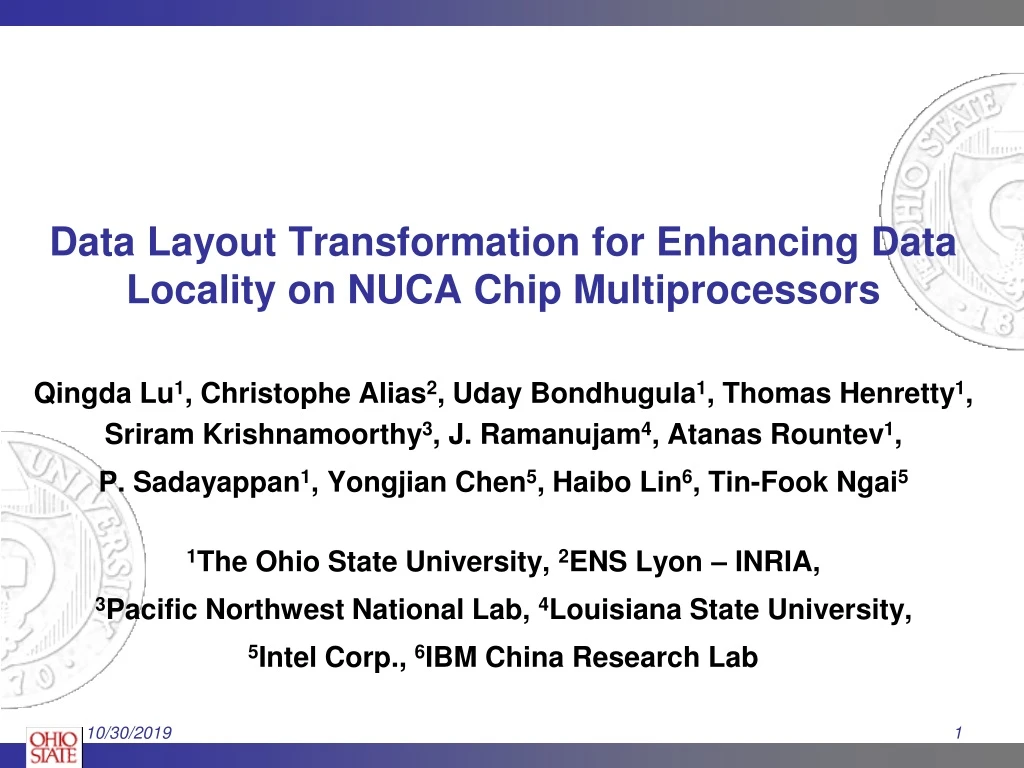
1. Data Layout Transformation for Enhancing Data Locality on NUCA Chip Multiprocessors Qingda Lu1, Christophe Alias2, Uday Bondhugula1, Thomas Henretty1, Sriram Krishnamoorthy3, J. Ramanujam4, Atanas Rountev1, P. Sadayappan1, Yongjian Chen5, Haibo Lin6, Tin-Fook Ngai5 1The Ohio State University, 2ENS Lyon – INRIA, 3Pacific Northwest National Lab, 4Louisiana State University, 5Intel Corp., 6IBM China Research Lab

2. The Hardware Trends • Trend of fabrication technology • Gate delay decreases • Wire delay increases • Trend of chip-multiprocessors (CMPs) • More processors • Larger caches • Private L1 cache • Shared last-level cache to reduce off-chip accesses • We focus on L2 cache

3. Physical Address Log2N bits Log2L bits Bank # Offset Non-Uniform Cache Architecture • The problem: Large caches have long latencies • The Solution • Employ a banked L2 cache organization with non-uniform latencies • NUCA designs • Static NUCA: Mapping of data into banks is predetermined based on the block index. • Dynamic NUCA: Migrating data among banks. Hard to implement due to overheads and design challenges.

4. T9 T6 T0 T1 T2 T3 T5 T8 T4 T10 T11 T12 T13 T14 T15 T7 Router Proc Private L1$ L2$ Bank Directory A Tiled NUCA-CMP

5. Motivating Example: Parallelizing 1D Jacobi on a 4-tile CMP • If we use the standard linear array layout and parallelize the program with the “owner-computes” rule, communication volume is roughly 2N cache lines in every outer iteration. • 1-D Jacobi Code: while (condition) { for (i = 1; i < N-1; i++) B[i] = A[i-1] + A[i] + A[i+1]; for (i = 1; i < N-1; i++) A[i] = B[i]; } Thread 0 Thread 1 Thread 2 Thread 3 A[0] A[1] A[8] A[9] A[16] A[17] A[24] A[25] A[2] A[3] A[10] A[11] A[18] A[19] A[26] A[27] A[4] A[5] A[12] A[13] A[20]A[21] A[28] A[29] A[6] A[7] A[14] A[15] A[22]A[23] A[30] A[31] B[0] B[1] B[8] B[9] B[16] B[17] B[24] B[25] B[2] B[3] B[10] B[11] B[18] B[19] B[26] B[27] B[4] B[5] B[12] B[13] B[20]B[21] B[28] B[29] B[6] B[7] B[14] B[15] B[22]B[23] B[30] B[31] Bank 0 Bank 1 Bank 2 Bank 3

6. Motivating Example: Parallelizing 1D Jacobi on a 4-tile CMP Thread 0 Thread 1 Thread 2 Thread 3 A[0] A[1] A[8] A[9] A[16] A[17] A[24] A[25] A[0] A[1] A[2] A[3] A[4] A[5] A[6] A[7] A[2] A[3] A[10] A[11] A[18] A[19] A[26] A[27] A[8] A[9] A[10] A[11] A[12] A[13] A[14] A[15] A[4] A[5] A[12] A[13] A[20]A[21] A[28] A[29] A[24] A[25] A[26] A[27] A[28] A[29] A[30] A[31] A[6] A[7] A[14] A[15] A[22]A[23] A[30] A[31] A[16] A[17] A[18] A[19] A[20] A[21] A[22] A[23] B[0] B[1] B[2] B[3] B[4] B[5] B[6] B[7] B[2] B[3] B[10] B[11] B[18] B[19] B[26] B[27] B[8] B[9] B[10] B[11] B[12] B[13] B[14] B[15] B[16] B[17] B[18] B[19] B[20] B[21] B[22] B[23] B[4] B[5] B[12] B[13] B[20]B[21] B[28] B[29] B[24] B[25] B[26] B[27] B[28] B[29] B[30] B[31] B[6] B[7] B[14] B[15] B[22]B[23] B[30] B[31] B[0] B[1] B[8] B[9] B[16] B[17] B[24] B[25] • If we divide the iteration space into four contiguous partitions and rearrange the data layout, only 6 remote cache lines are requested in every outer iteration. Bank 0 Bank 1 Bank 2 Bank 3

7. The Approach • A general framework for integrated data layout transformation and loop transformations for enhancing data locality on NUCA CMP’s • Formalism: polyhedral model • Two main steps: • Localization analysis: search for an affine mapping of iteration spaces and data spaces such that no iteration accesses any data that is beyond a bounded distance in the target space • Code generation: generate efficient indexing code using CLooG by differentiating the “bulk” scenario from the “boundary” case via linear constraints.

8. Polyhedral Model • An algebraic framework for representing affine programs – statement domains, dependences, array access functions – and affine program transformations • Regular affine programs • Dense arrays • Loop bounds – affine functions of outer loop variables, constants and program parameters • Array access functions - affine functions of surrounding loop variables, constants and program parameters

9. Polyhedral Model j≥2 j≤6 i i≤7 1 0 -1 ij1 . -1 0 7 DS1 (xS1)= 0 1 -2 i≥1 0 -1 6 ≥ 0 i j j 1 0 0 1 . 0 -1 + ₣S1,a(xS1)= for (i=1; i<=7; i++) for (j=2; j<=6; j++) S1: a[i][j] = a[j][i] + a[i][j-1]; i j xS1=

10. Computation Allocation and Data Mapping . . CS GA πS (xS)= ψA (XA )= • Computation allocation: • Original iteration space => Integer vector representing the virtual processor space • A one-dimensional affine transform (π) for a statement S is given by • Data Mapping: • Original data space => Integer vector representing the virtual processor space • A one-dimensional affine transform (ψ) for an array A is given by xSn 1 xAn 1

11. Localized Computation Allocation and Data Mapping • Definition: For a program P, let D be its index set, computation allocation π and data mapping ψ for P are localized if and only if for any array A, and any reference FS,A, , whereqis a constant. • As a special case, communication-free localization can be achieved if and only if for any array A and any array reference FS,A in a statement S, computation allocation π and data mapping ψ satisfy

12. Localization Analysis • Step 1: Group Interrelated Statements/Arrays • Form a bipartite graph: vertices corresponds to statements / arrays and edges connect each statement vertex to its referenced arrays. • Find the connected components in the bipartite graph. • Step 2: Find Localized Computation Allocation / Data Mapping for each connected component • Formulate the problem as finding an affine computation allocation π and an affine data mapping ψ that satisfy for every array reference FS,A • Translate the problem to a linear programming problem that minimizes q.

13. Localization Analysis Algorithm Require: Array access functions are rewritten to access byte arrays C = ∅ for each array reference FS,Ado Obtain new constraints: under and Apply Farkas Lemma to new constraints to obtain linear constraints; eliminate all Farkas multipliers Add linear inequalities from the previous step into C Add objective function (min q) Solve the resulting linear programming problem with constraints in C if ψ and π are found then return π, ψ, and q else return “not localizable”

14. Data Layout Transformation • Strip-mining • An array dimension N  two virtual dimensions • Array reference array reference [...][i][...]  [...][ i / d ][i mod d][...] • Permutation • Array A(...,N1, ...,N2, ...)  A’(...,N2, ...,N1, ...) • Array reference A[...][i1][...][i2][...]  A[...][i1][...][i2][...].

15. Data Layout Transformation (Cont.) A[0] A[1] A[8] A[9] A[16] A[17] A[24] A[25] A[2] A[3] A[10] A[11] A[18] A[19] A[26] A[27] A[4] A[5] A[12] A[13] A[20]A[21] A[28] A[29] A[6] A[7] A[14] A[15] A[22]A[23] A[30] A[31] B[0] B[1] B[8] B[9] B[16] B[17] B[24] B[25] B[2] B[3] B[10] B[11] B[18] B[19] B[26] B[27] B[4] B[5] B[12] B[13] B[20]B[21] B[28] B[29] B[6] B[7] B[14] B[15] B[22]B[23] B[30] B[31] • The 1D jacobi example: • Combination of strip-mining and permutation A[0] A[1] A[2] A[3] A[4] A[5] A[6] A[7] A[8] A[9] A[10] A[11] A[12] A[13] A[14] A[15] A[24] A[25] A[26] A[27] A[28] A[29] A[30] A[31] A[16] A[17] A[18] A[19] A[20] A[21] A[22] A[23] B[0] B[1] B[2] B[3] B[4] B[5] B[6] B[7] B[8] B[9] B[10] B[11] B[12] B[13] B[14] B[15] B[16] B[17] B[18] B[19] B[20] B[21] B[22] B[23] B[24] B[25] B[26] B[27] B[28] B[29] B[30] B[31] Bank 0 Bank 1 Bank 2 Bank 3

16. Data Layout Transformation(Cont.) • Padding: • Inter-array padding: keep the base addresses of arrays aligned to a tile specified by the data mapping function • Intra-array padding: align elements inside an array with “holes” to make a strip-mined dimension divisible by its sub-dimensions

17. Data Layout Transformation (Cont.) With localized computation allocation and data mapping: • If we find communication-free allocation with all arrays share the same stride along the fastest varying dimension, only padding is applied • Otherwise we create a blocked view of n-dimensional array A along dimension k with data layout transformations • If K=1, we have data layout transformation σ(in, in−1, ..., i2, i1 )= (in, in−1, ..., i2, (i1 mod(N1 /P))/L, i1 /(N1 /P), i1 mod L), L is cache line size in elements and P is processor number. • If K>1, we have data layout transformation, σ(in, in−1, ..., i2, i1 )= (in, ..., i1 /L, ikmod (Nk/ P)..., i2, ik/(Nk/P), i1 mod L).

18. Code Generation • It is challenging to generate efficient code • Replacing array reference A[u(i))] with A’[σ(u(i))] produces very inefficient code • We iterate directly in the data space of the transformed array. • In the polyhedral model, we specify an iteration domain D and an affine scheduling function for each statement. • Efficient code is then generated by CLooG that implements the Quilleré-Rajopadhye-Wilde algorithm.

19. Code Generation (Cont.) Key techniques used in generating code accessing layout transformed arrays • While σ is not affine, σ-1is. We replace constraints jk= σ(uk(i)) byσ-1 (jk) =i. • We separate the domain D into two sub-domains Dsteadyand Dboundaryand generate code for two domains. • Dsteadycovers the majority of D by simplifying constraints such as (i-u) mod L to (i mod L) – u • Boundary cases are automatically handled in Dboundary= D - Dsteady

20. Experimental Setup • With the VirtutechSimics full-system simulator extended with a timing infrastructure GEMS, we simulated a tiled NUCA-CMP: • We evaluated our approach with a set of data-parallel benchmarks • Focus of the approach is not on finding parallelism

21. Data Locality Optimization for NUCA-CMPs: The Results Speedup

22. Data Locality Optimization for NUCA-CMPs: The Results Link Utilization

23. Data Locality Optimization for NUCA-CMPs: The Results Remote L2 Access Number

24. Conclusion • We believe that the approach developed in this study provides very general treatment of code generation for data layout transformation • analysis of data access affinities • automated generation of efficient code for the transformed layout