Download
1 / 71
710 likes | 826 Views
Lecture 3. Global models: Towards modeling plate tectonics. Global surface observables Major ingredients of plate tectonics Linking mantle convection and lithospheric deformations. Key questions. How weak are the plate boundaries? How weak is asthenosphere ?

E N D
Lecture 3. Global models: Towards modeling plate tectonics • Global surface observables • Major ingredients of plate tectonics • Linking mantle convection and lithospheric deformations
Key questions • How weak are the plate boundaries? • How weak is asthenosphere? • How to make plate boundaries?
Spherical harmonic expansion Modified from website Of Svetlana Panasyuk
Spherical Harmonics Example Components for Degree (L) = 8 Zonal (m=0) Sectoral (m=L) Tesseral ( m=L/2)
Geoid • Measured by modelling satellite orbits. • Spherical harmonic representation, L=360. Range +/- 120 meters From, http://www.vuw.ac.nz/scps-students/phys209/modules/mod8.htm
Free-Air Gravity • Derivative of geoid (continents) • Measured over the oceans using satellite altimetry (higher resolution).
Free-Air Gravity • Derivative of geoid (continents) • Measured over the oceans using satellite altimetry (higher resolution).
Geoid/Free-air Gravity Spectra • L = 2-3 • very long wavelength • > 13,000 km • L = 60-360 • short wavelength. • 600-110 km. Red Spectrum Dominated by signal at long wavelengths • L = 4-12 • long wavelength • 10000-3000 km
Dynamic Topography Isostatically Compensated Dynamically Supported
Post-Glacial Rebound (PGR) • Glacial Isostatic Adjustment (GIA). • returning to isostatic equilibrium. • Unloading of the surface as ice melts (rapidly). From: http://www.pgc.nrcan.gc.ca/geodyn/ docs/rebound/glacial.html
Plate Motion • Well-known for the present time. • Accuracy degrades for times further in the past. Data: Argus & Gordon 1991 (NUVEL-NNR), Figure: T. Becker
Summary of Surface Observations Observation Quality . Post Glacial Rebound variable (center) Plate Motion good (recent) Geoid good (<100 km) Free-air Gravity good (shallow) Dynamic Topography poor (magnitude)
Plate Motion Observed plate velocities in no-net-rotation (NNR) reference frame
Plate Motion … and observed net-rotation (NR) of the lithosphere Based on analyses of seismic anisotropy Becker (2008) narrowed possible range of angular NR velocities down to 0.12-0.22 °/Myr
Full system of equations Full set of equations energy
Simplifying... Full set of equations mass energy
Simplified system of equations Full set of equations energy
Stokes equations Full set of equations Main tool to model mantle convection Solution is most simple if viscosity depends only on depth energy
Simplifying... Full set of equations mass
Mantle convection Solving Stokes equations with FE code Terra (Bunge et al.)
Ingredients of plate tectonics Convection (FE code Terra) Weak plate boundaries Ricard and Vigny, 1989; Bercovici, 1993; Bird, 1998; Moresi and Solomatov, 1998;Tackley, 1998, Zhong et al, 1998; Trompert and Hansen, 1998;Gurnis et al., 2000….
Ingredients of plate tectonics Generating plate boundaries Bercovici, 1993,1995, 1996, 1998, 2003; Tackley, 1998, 2000; Moresi and Solomatov, 1998; Zhong et al, 1998; Gurnis et al., 2000… Increasing yield stress Tendency: towards more realistic strongly non-linear rheology Viscous rheology-only and emulation of brittle failure van Heck and Tackley, 2008
Solving Stokes equations with code Rhea (adaptive mesh refinement) Burstedde et al.,2008-2010
Solving Stokes equations with code Rhea Stadler et al., 2010
Point 1 Global models can not generate yet present-day plates and correctly reproduce plate motions They employ plastic (brittle) rheolgical models inconsistent with laboratory data They can not also reproduce realistic one-sided subduction and pure transform boundaries
Modeling deformation at plate boundaries Dead Sea Transform Subduction and orogeny in Andes (Sobolev et al., EPSL 2005, Petrunin and Sobolev, Geology 2006, PEPI, 2008). Sobolev and Babeyko, Geology 2005; Sobolev et al., 2006
„Realistic“ rheology Balance equations Deformation mechanisms Mohr-Coulomb Popov and Sobolev ( PEPI, 2008)
Three creep processes Diffusion creep Peierls Dislocation creep Dislocation Peierls creep Diffusion ( Kameyama et al. 1999)
Coupling mantle convection and lithospheric deformation Lithospheric code (Finite Elements) Mantle code (spectral or FEM) Mantle and lithospheric codes are coupled through continuity of velocities and tractions at 300 km. Sobolev, Popov and Steinberger, in preparation
Above 300 km depth 3D temperature from surface heat flow at continents and ocean ages in oceans, crustal structure from model crust2.0 Below 300 km depth Spectral method (Hager and O’Connell,1981) with radial viscosity and 3D density distributions based on subduction history (Steinberger, 2000)
Mantle rheology olivine rheology with water content as model parameter Parameters in reference model by Hirth and Kohlstedt (2003) with n=3.5 +-0.3.
Plate boundaries Plate boundaries are defined as narrow zones with visco-plastic rheology where friction coefficient is model parameter
Lithospheric code (FEM) Mantle code (spectral) Mantle and lithospheric codes are coupled through continuity of velocities and tractions at 300 km. The model has free surface and 3D, strongly non-linear visco-elastic rheology with true plasticity (brittle failure) in upper 300km.
Benchmark test
Our model vrs. model by Becker (2006) (CitcomS) = 0.19 Misfit=
Effect of strength at plate boundaries Friction at boundaries 0.4 (Smax=600 MPa)
Friction at boundaries 0.1 (Smax=150 MPa) much too low velocities
Friction at boundaries 0.05 (Smax=75 MPa) too low velocities
Friction at boundaries 0.02 (Smax= 30 MPa) about right magnitudes of velocities
Friction at boundaries 0.01 (Smax= 15 MPa) too high velocities
Point 2 Strength (friction) at plate boundaries must be very low (<0.02), much lower than measured friction for any dry rock (>0.1) No high pressure fluid=no plate tectonics
Mantle rheology olivine rheology with water content as model parameter Parameters in reference model by Hirth and Kohlstedt (2003) with n=3.5 +-0.3.
Modeling scheme For every trial rheology (water content in asthenosphere) we calculate plate velocities for different frictions at plate boundaries, until we get best fit of observed plate velocities in the NNR reference frame Next, we look how well those optimized models actually fit observations
Lithospheric net rotation Becker (2008) Hirth and Kohlstedt (1996)