Download
1 / 55
550 likes | 681 Views
CHAPTER 14 Cash Flow Estimation and Risk Analysis. Relevant cash flows Working capital treatment Inflation Risk Analysis: Sensitivity Analysis, Scenario Analysis, and Simulation Analysis. Proposed Project. Cost: $200,000 + $10,000 shipping + $30,000 installation. Depreciable cost $240,000.

E N D
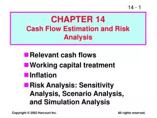
CHAPTER 14 Cash Flow Estimation and Risk Analysis • Relevant cash flows • Working capital treatment • Inflation • Risk Analysis: Sensitivity Analysis, Scenario Analysis, and Simulation Analysis
Proposed Project • Cost: $200,000 + $10,000 shipping + $30,000 installation. • Depreciable cost $240,000. • Inventories will rise by $25,000 and payables will rise by $5,000. • Economic life = 4 years. • Salvage value = $25,000. • MACRS 3-year class.
Incremental gross sales = $250,000. • Incremental cash operating costs = $125,000. • Tax rate = 40%. • Overall cost of capital = 10%.
Set up without numbers a time line for the project CFs. 0 1 2 3 4 Initial Outlay OCF1 OCF2 OCF3 OCF4 + Terminal CF NCF0 NCF1 NCF2 NCF3 NCF4
Incremental Cash Flow = Corporate cash flow withproject minus Corporate cash flow without project
Should CFs include interest expense? Dividends? • NO. The costs of capital are already incorporated in the analysis since we use them in discounting. • If we included them as cash flows, we would be double counting capital costs.
Suppose $100,000 had been spent last year to improve the production line site. Should this cost be included in the analysis? • NO. This is a sunk cost. Focus on incremental investment and operating cash flows.
Suppose the plant space could be leased out for $25,000 a year. Would this affect the analysis? • Yes. Accepting the project means we will not receive the $25,000. This is an opportunity cost and it should be charged to the project. • A.T. opportunity cost = $25,000 (1 - T) = $15,000 annual cost.
If the new product line would decrease sales of the firm’s other products by $50,000 per year, would this affect the analysis? • Yes. The effects on the other projects’ CFs are “externalities”. • Net CF loss per year on other lines would be a cost to this project. • Externalities will be positive if new projects are complements to existing assets, negative if substitutes.
Net Investment Outlay at t = 0 (000s) NWC = $25,000 - $5,000 = $20,000.
Depreciation Basics Basis = Cost + Shipping + Installation $240,000
What if you terminate a project before the asset is fully depreciated? Cash flow from sale = Sale proceeds - taxes paid. Taxes are based on difference between sales price and tax basis, where: Basis = Original basis - Accum. deprec.
Example: If Sold After 3 Years (000s) • Original basis = $240. • After 3 years = $17 remaining. • Sales price = $25. • Tax on sale = 0.4($25-$17) = $3.2. • Cash flow = $25-$3.2=$21.7.
Project Net CFs on a Time Line 0 1 2 3 4 (260)* 107 118 89 117 Enter CFs in CFLO register and I = 10. NPV = $81,573. IRR = 23.8%. *In thousands.
What is the project’s MIRR? (000s) 0 1 2 3 4 (260)* 107 118 89 117.0 97.9 142.8 142.4 500.1 (260) MIRR = ?
Calculator Solution 1. Enter positive CFs in CFLO:I = 10; Solve for NPV = $341.60. 2. Use TVM keys: PV = 341.60, N = 4I = 10; PMT = 0; Solve for FV = 500.10. (TV of inflows) 3. Use TVM keys: N = 4; FV = 500.10;PV = -260; PMT= 0; Solve for I = 17.8. MIRR = 17.8%.
What is the project’s payback? (000s) 0 1 2 3 4 (260)* (260) 107 (153) 118 (35) 89 54 117 171 Cumulative: Payback = 2 + 35/89 = 2.4 years.
If 5% inflation is expected over the next 5 years, are the firm’s cash flow estimates accurate? • No. Net revenues are assumed to be constant over the 4-year project life, so inflation effects have not been incorporated into the cash flows.
Real vs. Nominal Cash flows • In DCF analysis, k includes an estimate of inflation. • If cash flow estimates are not adjusted for inflation (i.e., are in today’s dollars), this will bias the NPV downward. • This bias may offset the optimistic bias of management.
What does “risk” mean in capital budgeting? • Uncertainty about a project’s future profitability. • Measured by NPV, IRR, beta. • Will taking on the project increase the firm’s and stockholders’ risk?
Is risk analysis based on historical data or subjective judgment? • Can sometimes use historical data, but generally cannot. • So risk analysis in capital budgeting is usually based on subjective judgments.
What three types of risk are relevant in capital budgeting? • Stand-alone risk • Corporate risk • Market (or beta) risk
How is each type of risk measured, and how do they relate to one another? 1. Stand-Alone Risk: • The project’s risk if it were the firm’s only asset and there were no shareholders. • Ignores both firm and shareholder diversification. • Measured by the or CV of NPV, IRR, or MIRR.
Probability Density Flatter distribution, larger , larger stand-alone risk. NPV 0 E(NPV) Such graphics are increasingly used by corporations.
2. Corporate Risk: • Reflects the project’s effect on corporate earnings stability. • Considers firm’s other assets (diversification within firm). • Depends on: • project’s , and • its correlation with returns on firm’s other assets. • Measured by the project’s corporate beta.
Profitability Project X Total Firm Rest of Firm 0 Years 1. Project X is negatively correlated to firm’s other assets. 2. If r < 1.0, some diversification benefits. 3. If r = 1.0, no diversification effects.
3. Market Risk: • Reflects the project’s effect on a well-diversified stock portfolio. • Takes account of stockholders’ other assets. • Depends on project’s and correlation with the stock market. • Measured by the project’s market beta.
How is each type of risk used? • Market risk is theoretically best in most situations. • However, creditors, customers, suppliers, and employees are more affected by corporate risk. • Therefore, corporate risk is also relevant.
Stand-alone risk is easiest to measure, more intuitive. • Core projects are highly correlated with other assets, so stand-alone risk generally reflects corporate risk. • If the project is highly correlated with the economy, stand-alone risk also reflects market risk.
What is sensitivity analysis? • Shows how changes in a variable such as unit sales affect NPV or IRR. • Each variable is fixed except one. Change this one variable to see the effect on NPV or IRR. • Answers “what if” questions, e.g. “What if sales decline by 30%?”
NPV (000s) Unit Sales Salvage 82 k -30 -20 -10 Base 10 20 30 Value
Results of Sensitivity Analysis • Steeper sensitivity lines show greater risk. Small changes result in large declines in NPV. • Unit sales line is steeper than salvage value or k, so for this project, should worry most about accuracy of sales forecast.
What are the weaknesses ofsensitivity analysis? • Does not reflect diversification. • Says nothing about the likelihood of change in a variable, i.e. a steep sales line is not a problem if sales won’t fall. • Ignores relationships among variables.
Why is sensitivity analysis useful? • Gives some idea of stand-alone risk. • Identifies dangerous variables. • Gives some breakeven information.
What is scenario analysis? • Examines several possible situations, usually worst case, most likely case, and best case. • Provides a range of possible outcomes.
Assume we know with certainty all variables except unit sales, which could range from 900 to 1,600. E(NPV) = $ 82 (NPV) = 47 CV(NPV) = (NPV)/E(NPV) = 0.57
If the firm’s average project has a CV of 0.2 to 0.4, is this a high-risk project? What type of risk is being measured? • Since CV = 0.57 > 0.4, this project has high risk. • CV measures a project’s stand-alone risk. It does not reflect firm or stockholder diversification.
Would a project in a firm’s core business likely be highly correlated with the firm’s other assets? • Yes. Economy and customer demand would affect all core products. • But each product would be more or less successful, so correlation < +1.0. • Core projects probably have corre-lations within a range of +0.5 to +0.9.
How do correlation and affecta project’s contribution tocorporate risk? • If P is relatively high, then project’s corporate risk will be high unless diversification benefits are significant. • If project cash flows are highly cor-related with the firm’s aggregate cash flows, then the project’s corporate risk will be high if P is high.
Would a core project in the furniture business be highly correlated with the general economy and thus with the “market”? • Probably. Furniture is a deferrable luxury good, so sales are probably correlated with but more volatile than the general economy.
Would correlation with the economy affect market risk? • Yes. • High correlation increases market risk (beta). • Low correlation lowers it.
With a 3% risk adjustment, should our project be accepted? • Project k = 10% + 3% = 13%. • That’s 30% above base k. • NPV = $60,541. • Project remains acceptable after accounting for differential (higher) risk.
Should subjective risk factors be considered? • Yes. A numerical analysis may not capture all of the risk factors inherent in the project. • For example, if the project has the potential for bringing on harmful lawsuits, then it might be riskier than a standard analysis would indicate.
Are there any problems with scenario analysis? • Only considers a few possible out-comes. • Assumes that inputs are perfectly correlated--all “bad” values occur together and all “good” values occur together. • Focuses on stand-alone risk, although subjective adjustments can be made.
What is a simulation analysis? • A computerized version of scenario analysis which uses continuous probability distributions. • Computer selects values for each variable based on given probability distributions. (More...)