Download
1 / 31
310 likes | 437 Views
Quantum-like Description of Data from Experiments on Prisoner’s Dilemma. Andrei Khrennikov International Center for Mathematical Modeling in Physics and Cognitive Sciences University of Växjö, Sweden. Law of total probability.

E N D
Quantum-like Description of Data from Experiments on Prisoner’s Dilemma Andrei Khrennikov International Center for Mathematical Modeling in Physics and Cognitive Sciences University of Växjö, Sweden
Law of total probability ``The prior probability to obtain the result e.g. b=+1 for the random variable b is equal to the prior expected value of the posterior probability of b=+1 under conditions a=+1 and a=-1.” • P(b=j)= P(a=+1) P(b=j |a=+1) +P(a=-1) P(b=j |a=-1), j=+1 or j=-1. It gives the possibility to predict the probabilities for the b-variable on the basis of conditional probabilities and the a-probabilities.
Violation of the formula of total probability • We point out that in the conventional probability theory this formula is derived for one fixed probability space. • It represents (see Kolmogorov) one fixed complex of experimental conditions -- one context. • It is natural to expect that in multi-contextual approach this formula can be violated
Author’s publications on violation of the formula of total probability Interpretations of Probability.VSP Int. Sc. Publishers, Utrecht/Tokyo, 1999 (second edition, 2004). Information dynamics in cognitive psychological, social, and anomalous phenomena. Kluwer, Dordreht, 2004. • Linear representations of probabilistic transformations induced by context transitions. J. Phys. A: Math. Gen., 34, 9965-9981 (2001). • Representation of the Kolmogorov model having all distinguishing features of quantum probabilistic model. Phys. Lett. A, 316, 279-296 (2003). • In Russian: A. Yu. Hrennikov, Nekolmogorovskie teorii veroyatnostei I ih prilojeniya k kvantovoi fizike, Moskva, Nauka, Fizmatlit
Contextual dependence of probabilities and interference term • If the formula of total probability does not hold true (as a consequence • of multi-contextuality), then the left-hand side does not equal to the • right-hand side. • We call this difference interference term by analogy with quantum • mechanics in which the formula of total probability is violated • inducing so called interference of probabilities. Given context C (physical, mental, financial). Observables a and b are measured producing probabilities: P(a=+1|C), P(a=-1|C), P(b=+1|C), P(b=-1|C), here, e.g., P(a=+1 |C) is the probability for a=+1 under C.
Selection-Contexts • First a-measurement is performed and combined with selections for the values a=+1 and a= -1. Two selection contexts, say C(a=+1) and C(a=-1), are created. For example, ”a” is a question asked to people. Here C(a=+1) produces the ensemble of people who replied ”yes” and C(a=-1) those who replied ”no.” • For selection-contexts C(a=+1) and C(a=-1), we perform the b-measurement and obtain the ”conditional probabilities” (contextual probabilities): P(b=+1| C(a=+1)), P(b=-1| C(a=+1)), P(b=+1|C(a=-1)), P(b=+1| C(a=-1)).
Contextual Form of the von Neumann Projection Postulate Measurement of the a-variable is also performed for some context, say C0. In principle, the selection contexts might remember the original context C0: C(a=+1)=C(a=+1|C0),C(a=-1)=C(a=-1|C0). Such C0-memory blocks the possibility to proceed by analogy with quantum probability. We assume that the effect of the a-measurement is so strong that it destroys memory. In fact, this postulate is a contextual version of vonNeumann’s postulate: projection on the eigenvector corresponding to obtained eigenstate of the quantum observable. If it holds, then the selection contexts C(a=+1), C(a=-1) do not depend on C0.
Formula of total probability with interference term • Contextual Projection Postulate: P(b=+1 |a=+1),…, P(b=-1|a=-1). • In contextual notations the interference terms are given by δ(b=+1|C)= P(b=+1|C) – [P(a=+1|C) P(b=+1|a=+1) - P(a=-1 | C) P(b=+1|a=-1)] δ(b=-1 |C)= P(b=-1|C) – [P(a=-1|C) P(b=-1|a=+1) - P(a=-1 | C) P(b=-1|a=-1)]. Thus: • P(b=j|C)= P(a=+1|C) P(b=j|a=+1) +P(a=-1|C) P(b=j|a=-1) + δ(b=j |C) By analogy with QM we select normalization: • λ = δ /2√P, where P= P(a=+1|C) P(b=j|a=+1)P(a=-1|C) P(b=j|a=-1)
Trigonometric and hyperbolic interference P(b=j|C)= P(a=+1 |C) P(b=j|C(a=+1)) - P(a=-1|C) P(b=j|C(a=-1)) + 2 λ(j) √P If the normalized interference term λ is less than 1, we can find such an angle φ that λ = cos φ; in the opposite case we can represent λ = εcosh φ, ε=+1 or -1. Here φ= φ(j |C): The ”probabilistic angle” depends on context C. The first case we call trigonometric interference and the second hyperbolic interference.
Trigonometric and hyperbolic interferences P(b=j|C)= P(a=+1|C) P(b=j|a=+1)+P(a=-1|C)P(b=j| a=-1)+2 cosφ(j)√P It can be easily derived in the formalism of QM by using the Born’s rule, i.e., reprsentation of probabilities by squares of complex amplitudes. But (!!!) we did not start with Hilbert space.Trigonometric interference was obtained starting with contextual probabilities. Interference terms of the hyperbolic form: λ = εcosh φ are not predicted by QM. • They appear naturally in the general contextual framework. • Is QM only a very special case of violation of the law of total probability? Can hyperbolic interference appear in cognitive science, economics? Even in physics?
QM restrictions on formula of total probability with intereference term • In QM the matrix of transition probabilities P(b=i | a=j) is very special -- DOUBLY STOCHASTIC: in a doubly stochastic matrix all columns sum to 1. • Can we expect that outside QM transition matrices would be always doubly stochastic? • Not at all: Conte, E., Todarello, O., Federici, A., Vitiello, F., Lopane, M., Khrennikov, A. Yu and Zbilut, J. P. (2006). Some remarks on an experiment suggesting quantum-like behavior of cognitive entities and formulation of an abstract quantum mechanical formalism to describe cognitive entity and its dynamics. Chaos, Solitons and Fractals, 31, 1076-1088.
Quantum-Like Representation Algorithm-- QLRA • If we have the collection of probabilities P(b=j|C), P(a=k |C), P(b=j|a=k), j, k=+1,-1, then we can find the angles of interference φ =φ(j|C). On the basis of this data we can construct the complex probability amplitude ψ(j)=ψ(j |C)representing the original context C on the basis of two dichotomous observables: a and b. Born’s rule take place: |ψ(j) |² = P(b=j|C). This is so called ”inverse Born’s problem”: To represent probabilistic data of any origin by probability amplitudes.
Quantum-Great menatl and social QL-conjecture • In the process of evolution cognitive and social systems developed the ability to create QL-representation and operate with probabilities in ”vector mental space.”
Quantum-like modeling of disjunction effects • J. Busemeyer, A. Lambert-Mogilanski, V. Danilov, A. Khrennikov found that disjunction effects in economics and social science could be described by QM or QL formalism. I shall perform QL-modeling of disjunction effects by representing statistical data from famous Tversky-Shafir and Shafir-Tversky experiments by complex (and hyperbolic) probability amplitudes. In particular, we find interference angles. PD is a game in which two players can cooperate with or defect (i.e. betray) the other player. The only concern of each individual player (prisoner) is maximizing own payoff. In simpler terms, no matter what the other player does, one player will always gain a greater payoff by playing defect. Since in any situation playing defect is more beneficial than cooperating, all rational players will play defect.
The classical PD • Two suspects, A and B, are arrested by the police. • The police have insufficient evidence for a conviction, and, having • separated both prisoners, visit each of them to offer the same deal: • if one testifies for the prosecution against the other and the other remains silent, the betrayer goes free and the silent accomplice receives the full 10-year sentence. • If both stay silent, both prisoners are sentenced to only six months in jail for a minor charge. • If each betrays the other, each receives a two-year sentence. • Each prisoner must make the choice of whether to betray the other or to remain silent. However, neither prisoner knows for sure what choice the other prisoner will make. So this dilemma poses the question: • How should the prisoners act?
Rational Behavior • The principle of rational behavior which is basic for rational choice theory which is the dominant theoretical paradigm in microeconomics. It is also central to modern political science and is used by scholars in other disciplines such as sociology. • However, Shafir and Tversky found that players frequently behave irrationally.
Contextual analysis of Prisoner's Dilemma • Context C represents the situation such that a player has no idea about planned action of another player. • Context C(a=+1) represents the situation such that the B-player supposes that A will cooperate and context C(a=-1) -- A will compete. We can also consider similar contexts C(b=+1), C(b=-1). • A priory the law of total probability might be violated for PD, since the B-player is not able to combine contexts. • If those contexts were represented by subsets of a so called space of ``elementary events'' as it is done in classical probability theory the B-player considers conjunction of the contexts C and e.g. C(a=+1) and to operate in this context. • But the very situation of PD is such that one could not expect that contexts C and C(a=+1) might be peacefully combined.
Shafir and Tversky PD experiment,1992, Cognitive Psychology, 24, 449-474. • P(b= -1 |C)=0.63 and hence P(b=+ 1|C)=0.37; • P(b=-1|a=-1) =0.97, P(b=+1|a=-1) =0.03; • P(b=-1|a=+1) =0.84, P(b=+1|a=+1) =0.16. • As always in probability theory it is convenient to introduce the matrix of transition probabilities P= • 0.16 0.84 • 0.03 0.97 It is not doubly stochastic! This data is quantum-like. It can be, nevertheless, represented by complex probability amplitude. Our QLRA works well even in such a case.
Tversky—Shafir gambling experiment, 1992, Psychological Science, 3, 305-309. • In this experiment, you are presented with two possible plays of a gamble that is equally likely to win 200 USD or lose 100USD. • You are instructed that the first play has completed, and now you are faced with the possibility of another play. • Here a gambling device, e.g., roulette, plays the role of A; • B is a real player, his actions are b=+1, to play the second game, b=-1, not. • Here the context C corresponds to the situation such that the result of the first game is unknown for B; the contexts C(a=±1) correspond to the situations such that the results a=±1 of the first play in the gamble are known.
Contextual description of Tversky—Shafir gambling experiment • From Tversky and Shafir, 1992, we have: • P(b=+1|C)=0.36 and hence P(b=-1|C)=0.64; • P(b=+1|a=-1)=0.59, P(b=-1|a=-1)=0.41; • P(b=+1|a=+1)=0.69, P(b=-1|a=+1)=0.31.
Coefficients of interference for disjunction experiments • 1. Since in the Tversky--Shafir gambling experiment the A-probabilities are fixed, it is easier for investigation. • Simple arithmetic calculations give δ(+1) = -0.28, and hence λ(+1) = -0.44. Thus the probabilistic phase • φ(+1) = 2.03. • We recall the general math. fact about the δ-coefficients • δ (+1)+ δ(-1)=0. • Thus δ(-1) = 0.28, and hence λ(-1)= 0.79. Thus the probabilistic phase • φ(-1) = 0.66.
In the case of Shafir--Tversky PD-experiment the B-player assigns probabilities of the A-actions, p and1-p. Thus coefficients of interference depends on p. • We start with δ(-1) = -(0.21 +0.13 p) and • λ(-1)= - (0.12 +0.07 p )/[p(1-p)]½. • We now find δ(+1) = (0.21 +0.13 p) and • λ(+1)=-(1.52 + 0.94 p)/[p(1-p)]½. • Suppose B assumes that A will acts with • p = 1-p =1/2. • Then the interference between contexts is given by λ(-1) = -0.31 and hence the phase φ(-1) = 1.89. But in such a situation λ(+1)=3.98! • The latter interference is very high. It exceeds the possible range of QM interference. This is the case of hyperbolic interference! Here the hyperbolic phase φ(+1)= 2.06.