Download
1 / 37
370 likes | 505 Views
CHAPTER 6 Statistical Inference & Hypothesis Testing . 6.1 - One Sample Mean μ , Variance σ 2 , Proportion π 6.2 - Two Samples Means, Variances, Proportions μ 1 vs. μ 2 σ 1 2 vs. σ 2 2 π 1 vs. π 2 6.3 - Multiple Samples Means, Variances, Proportions

E N D
CHAPTER 6Statistical Inference & Hypothesis Testing 6.1 - One Sample Mean μ, Variance σ2, Proportion π 6.2 - Two Samples Means, Variances, Proportions μ1vs.μ2σ12vs.σ22π1vs.π2 6.3 - Multiple Samples Means, Variances, Proportions μ1, …, μkσ12, …,σk2π1, …, πk
CHAPTER 6Statistical Inference & Hypothesis Testing 6.1 - One Sample Mean μ, Variance σ2, Proportion π 6.2 - Two Samples Means, Variances, Proportions μ1vs.μ2σ12vs.σ22π1vs.π2 6.3 - Multiple Samples Means, Variances, Proportions μ1, …, μkσ12, …,σk2π1, …, πk
Binary Response: P(Success) = “Test of Homogeneity” POPULATION TWO POPULATIONS Two random binary variables I and J Random binary variable I I = 1 I = 0 “Do you like olives?” “Do you like Brussel sprouts?” = P(Yes to Brussel sprouts) Null Hypothesis H0: 1=2 “No difference in liking Brussel sprouts between two pops.” Alternative Hypothesis HA: 1 ≠ 2 “There is a difference in liking Brussel sprouts bet two pops.”
Binary Response: P(Success) = “Test of Homogeneity” POPULATION TWO POPULATIONS Two random binary variables I and J Random binary variable I J = 1 J = 0 “Do you like anchovies?” “Do you like Brussel sprouts?” = P(Yes to Brussel sprouts) Null Hypothesis H0: 1=2 “No difference in liking Brussel sprouts between two pops.” Alternative Hypothesis HA: 1 ≠ 2 “There is a difference in liking Brussel sprouts bet two pops.”
Binary Response: P(Success) = “Test of Independence” “Test of Homogeneity” POPULATION TWO POPULATIONS Two random binary variables I and J Random binary variable I I = 1 I = 0 J = 1 J = 0 “Do you like olives?” “Do you like anchovies?” “Do you like Brussel sprouts?” 2 = P(Yes to olives, given No to anchovies) 1 = P(Yes to olives, given Yes to anchovies) = P(Yes to Brussel sprouts) Null Hypothesis H0: 1=2 “No association exists between liking olives and anchovies.” Null Hypothesis H0: 1=2 “No difference in liking Brussel sprouts between two pops.” Alternative Hypothesis HA: 1 ≠ 2 “An association exists between liking olives and anchovies.” Alternative Hypothesis HA: 1 ≠ 2 “There is a difference in liking Brussel sprouts bet two pops.”
Binary Response: P(Success) = “Test of Independence” “Test of Homogeneity” POPULATION TWO POPULATIONS Two random binary variables I and J Random binary variable I I = 1 I = 0 J = 1 J = 0 “Do you like olives?” “Do you like anchovies?” “Do you like Brussel sprouts?” 2 = P(Yes to olives, given No to anchovies) 1 = P(Yes to olives, given Yes to anchovies) = P(Yes to Brussel sprouts) Sample, size n1 Sample, size n2 Sample, size n1 Sample, size n2 (Assume “large” sample sizes.)
Sample 1, size n1 Sample 2, size n2 X1 = # Successes X2 = # Successes Sampling Distribution of Problem:s.e. depends on !! Recall… Ifn 15 and n (1 – ) 15, then via the Normal Approximation to the Binomial… Solution: Use Ifn 15 and n (1 – ) 15, then via the Normal Approximation to the Binomial…
Sample 1, size n1 Sample 2, size n2 X1 = # Successes X2 = # Successes Ifn22 15 and n2 (1 – 2) 15, then via Normal Approximation to the Binomial Ifn11 15 and n1 (1 – 1) 15, then via Normal Approximation to the Binomial Sampling Distribution of Recall from section 4.1 (Discrete Models): Mean(X – Y) = Mean(X) – Mean(Y) and if X and Y are independent… Var(X – Y) = Var(X) + Var(Y)
Sample 1, size n1 Sample 2, size n2 X1 = # Successes X2 = # Successes “Null Distribution” standard error Similar problem as “one proportion” inference s.e.! = 0 under H0 Sampling Distribution of • For confidence interval, replace 1 and 2 respectively, by • For critical regionand p-value, replace 1 and 2 respectively, by….. ???? Null Hypothesis H0: 1=2 standard error estimate …so replace their common value by a “pooled” estimate. 0
Example: Two Proportions (of “Success”) • Study Question: “Is there an association between liking Bruce Willis movies and gender, or not?”
Example: Two Proportions (of “Success”) • Study Question: “Is there an association between liking Bruce Willis movies and gender, or not?” Test of Homogeneity (between two populations) Test of Homogeneity or Independence? • Design: Randomly select two large samples of males and females, and record their binary responses (Yes = 1, No = 0) to the question “Do you like Bruce Willis movies?” • Let the discrete random variableX = “# Successes” (i.e., “Yes” responses) in each gender of the samples, and use these data to test… • Null Hypothesis H0: P(“Yes” among Males) = P(“Yes” among Females), i.e., • Analysis via Z-test: Point estimates π1– π2 = 0, H0: π1= π2where π = P(Success) in each gender population. “No association exists.” • Data: Sample 1)n1 = 60 males, X1 = 42 Sample 2)n2 = 40 females, X2 = 16 NOTE: This is > 0. Therefore, REJECT H0 Conclusion: A significant association exists at the .05 level between “liking Bruce Willis movies” and gender, with males showing a 30% preference over females, on average.
Example: Two Proportions (of “Success”) • Study Question: “Is there an association between liking Bruce Willis movies and gender, or not?” Test of Homogeneity or Independence • Design: Randomly select two large samples of males and females, and record their binary responses (Yes = 1, No = 0) to the question “Do you like Bruce Willis movies?” • Let the discrete random variableX = “# Successes” (i.e., “Yes” responses) in each gender of the samples, and use these data to test… • Null Hypothesis H0: P(“Yes” among Males) = P(“Yes” among Females), i.e., • Analysis via Z-test: Point estimates π1– π2 = 0, H0: π1= π2where π = P(Success) in each gender population. “No association exists.” • Data: Sample 1)n1 = 60 males, X1 = 42 Sample 2)n2 = 40 females, X2 = 16 NOTE: This is > 0. Therefore, REJECT H0 Conclusion: A significant association exists at the .05 level; “liking Bruce Willis movies” and gender are dependent, with males showing a 30% preference over females, on average.
Binary Response: P(Success) = “Test of Independence” “Test of Homogeneity” POPULATION TWO POPULATIONS Two random binary variables I and J Random binary variable I I = 1 I = 0 J = 1 Males Females J = 0 “Do you like olives?” “Do you like anchovies?” “Do you like Bruce Willis movies?” 2 = P(Yes to olives, given No to anchovies) 1 = P(Yes to olives, given Yes to anchovies) = P(Yes to Bruce Willis movies) Null Hypothesis H0: 1=2 “No association exists between liking olives and anchovies.” Null Hypothesis H0: 1=2 “No difference in liking Bruce Willis between two pops.” Alternative Hypothesis HA: 1 ≠ 2 “An association exists between liking olives and anchovies.” Alternative Hypothesis HA: 1 ≠ 2 “There is a difference in liking Bruce Willis bet two pops.”
Binary Response: P(Success) = “Test of Independence” “Test of Homogeneity” POPULATION TWO POPULATIONS Two random binary variables I and J Random binary variable I I = 1 I = 0 J = 1 Males Females J = 0 “Do you like olives?” “Do you like Bruce Willis?” “Gender: Male?” “Do you like anchovies?” “Do you like Bruce Willis movies?” 2 = P(Yes to Bruce, given No to Male = Female) 1 = P(Yes to Bruce, given Yes to Male) = P(Yes to Bruce Willis movies) Null Hypothesis H0: 1=2 “No association exists between liking Bruce and gender.” Null Hypothesis H0: 1=2 “No difference in liking Bruce Willis between two pops.” Alternative Hypothesis HA: 1 ≠ 2 “An association exists between liking Bruce and gender.” Alternative Hypothesis HA: 1 ≠ 2 “There is a difference in liking Bruce Willis bet two pops.”
Example: Two Proportions (of “Success”) • Study Question: “Is there an association between liking Bruce Willis movies and gender, or not?” • Design: Randomly select two large samples of males and females, and record their binary responses (Yes = 1, No = 0) to the question “Do you like Bruce Willis movies?” • Let the discrete random variableX = “# Successes” (i.e., “Yes” responses) in each gender of the samples, and use these data to test… • Null Hypothesis H0: P(“Yes” among Males) = P(“Yes” among Females), i.e., π1– π2 = 0, H0: π1= π2where π = P(Success) in each gender population. “No association exists.” • Data: Sample 1)n1 = 60 males, X1 = 42 Sample 2)n2 = 40 females, X2 = 16 ~ ALTERNATE METHOD ~ I = 1 I = 0 J = 1 J = 0
Example: Two Proportions (of “Success”) • Study Question: “Is there an association between liking Bruce Willis movies and gender, or not?” • Design: Randomly select two large samples of males and females, and record their binary responses (Yes = 1, No = 0) to the question “Do you like Bruce Willis movies?” • Let the discrete random variableX = “# Successes” (i.e., “Yes” responses) in each gender of the samples, and use these data to test… • Null Hypothesis H0: P(“Yes” among Males) = P(“Yes” among Females), i.e., π1– π2 = 0, H0: π1= π2where π = P(Success) in each gender population. “No association exists.” • Data: Sample 1)n1 = 60 males, X1 = 42 Sample 2)n2 = 40 females, X2 = 16 Observed Expected (under H0)
Recall Probability Tables from Chapter 3…. Under the null hypothesis, the binary variable I is statistically independent of the binary variable J, i.e., P(I∩ J) = P(I)P(J).
Recall Probability Tables from Chapter 3…. Under the null hypothesis, the binary variable I is statistically independent of the binary variable J, e.g., P(“I = 1” ∩ “J = 1”) = P(“I = 1”)P(“J = 1”). Contingency Table Probability Table Therefore… , etc.
Example: Two Proportions (of “Success”) • Study Question: “Is there an association between liking Bruce Willis movies and gender, or not?” • Design: Randomly select two large samples of males and females, and record their binary responses (Yes = 1, No = 0) to the question “Do you like Bruce Willis movies?” • Let the discrete random variableX = “# Successes” (i.e., “Yes” responses) in each gender of the samples, and use these data to test… • Null Hypothesis H0: P(“Yes” among Males) = P(“Yes” among Females), i.e., π1– π2 = 0, H0: π1= π2where π = P(Success) in each gender population. “No association exists.” • Data: Sample 1)n1 = 60 males, X1 = 42 Sample 2)n2 = 40 females, X2 = 16 Observed “Chi-squared” Test Statistic Expected (under H0) Check: Is the null hypothesis true? 23.2 34.8 where “degrees of freedom” df = (# rows – 1)(# cols – 1), = 1 for a 2 2 table. 25.2 16.8
Example: Two Proportions (of “Success”) • Study Question: “Is there an association between liking Bruce Willis movies and gender, or not?” • Design: Randomly select two large samples of males and females, and record their binary responses (Yes = 1, No = 0) to the question “Do you like Bruce Willis movies?” Expected (under H0) Observed “Chi-squared” Test Statistic p = ????? = 8.867 on 1 df
Because 8.867 is much greater than the α=.05 critical value of 3.841, it follows that p << .05. More precisely, 7.879 < 8.867 < 9.141; hence .0025 < p < .005. α=.05 Yes = c(42, 16) No = c(18, 24) Bruce = rbind(Yes, No) chisq.test(Bruce, correct = F) The actual p-value = .0029, the same as that found using the Z-test! Pearson's Chi-squared test data: Bruce X-squared = 8.867, df = 1, p-value = 0.002904
Example: Two Proportions (of “Success”) • Study Question: “Is there an association between liking Bruce Willis movies and gender, or not?” • Design: Randomly select two large samples of males and females, and record their binary responses (Yes = 1, No = 0) to the question “Do you like Bruce Willis movies?” Expected (under H0) Observed “Chi-squared” Test Statistic The α=.05 critical value is 3.841. p = .0029 Recall… = 8.867 on 1 df
Example: Two Proportions (of “Success”) • Study Question: “Is there an association between liking Bruce Willis movies and gender, or not?” • Design: Randomly select two large samples of males and females, and record their binary responses (Yes = 1, No = 0) to the question “Do you like Bruce Willis movies?” • Let the discrete random variableX = “# Successes” (i.e., “Yes” responses) in each gender of the samples, and use these data to test… • Null Hypothesis H0: P(“Yes” in Male population) = P(“Yes” in Female population), i.e., • Analysis via Z-test: Point estimates π1– π2 = 0, H0: π1= π2where π = P(Success) in each gender population. “No association exists.” • Data: Sample 1)n1 = 60 males, X1 = 42 Sample 2)n2 = 40 females, X2 = 16 NOTE: This is > 0. Therefore, REJECT H0 Conclusion: A significant association exists at the .05 level; “liking Bruce Willis movies” and gender are dependent, with males showing a 30% preference over females, on average.
Example: Two Proportions (of “Success”) • Study Question: “Is there an association between liking Bruce Willis movies and gender, or not?” • Design: Randomly select two large samples of males and females, and record their binary responses (Yes = 1, No = 0) to the question “Do you like Bruce Willis movies?” Expected (under H0) Observed “Chi-squared” Test Statistic The α=.05 critical value is 3.841. p = .0029 = 8.867 on 1 df NOTE:(Z-score)2 = (2.9775)2 = 8.867 on 1 df NOTE:(Z-score)2 = (2.9775)2 Connection between Z-test and Chi-squared test ! Connection between Z-test and Chi-squared test !
“Chi-squared” Test Statistic for Categorical Data “degrees of freedom” df = (# rows – 1)(# cols – 1) • 2 2 Chi-squared Test is only valid if: • Null Hypothesis H0: 1 – 2 = 0. One-sided or nonzero null value Z-test! • Expected Values 5, in order to avoid “spurious significance” due to a possibly inflated Chi-squared value. • Paired version of 2 2 Chi-squared Test = McNemar Test • Categorical data – contingency table with any number of rows and columns • Formal Null Hypothesis difficult to write mathematically in terms of 1, 2,… • “Test of Independence” “Test of Homogeneity” • Informal H0: “No association exists between rows and columns.” • 80% of Expected Values 5 • See notes for other details, comments, including “Goodness-of-Fit” Test.