Download
1 / 48
480 likes | 600 Views
Statistics Workshop Concepts of Probability J-Term 2009 Bert Kritzer. Why Probability?. Statistical Inference seeks to separate what is observed into “systematic” and “random” components Observation = Systematic + Random

E N D
Statistics Workshop Concepts of ProbabilityJ-Term 2009Bert Kritzer
Why Probability? • Statistical Inference seeks to separate what is observed into “systematic” and “random” components Observation = Systematic + Random • Inference about characteristics of a “population” using information from a random sample • Estimating of population “parameters” • Nonrandom samples: the Literary Digest predicts Landon in a landslide • Inference about processes: random vs. systematic • Inference using population data
Defining and Expressing Probability • Definition: the proportion in the long run • a priori • empirical • subjective • Representing probability • as a proportion between 0 and 1 (p orπ) • as an odds (Ω)
Multiplication RuleIndependent Events Head on first toss and tail on second toss:
Addition RuleExclusive Events One tail on two tosses:
⅓ E EEE E ĒEEĒ ⅔ ⅓ E EĒE E ⅓ ⅓ ⅓ ⅔ ⅔ ⅔ ⅔ ĒEĒĒ ⅔ E ĒEE ⅓ E ⅓ ⅔ ⅔ ĒĒEĒ ⅔ ⅓ E ĒĒE ⅔ Ē ⅔ Ē ĒĒĒ Three Dice Rolls E = Probability of a 1 or a 2 Ē Ē
General Addition Rule G = heart H = face card ♥ A 2 3 4 5 6 7 8 9 10 J Q K ♦ A 2 3 4 5 6 7 8 9 10 J Q K ♠ A 2 3 4 5 6 7 8 9 10 J Q K ♣ A 2 3 4 5 6 7 8 9 10 J Q K
Conditional Probability Probability that an event A will occur given (|) that event B has already occurred Probability of A conditional B having aleady occurred
General Multiplication Rule From this we can see
Statistical Independence An event F is called statistically independent of an event E if, and only if: Coin flips: P(Head|Head) = P(Head) Card deck cut: P(Ace|Ace) = P(Ace) Dealt cards: P(Ace|Ace) ≠P(Ace)
Multiplication Rule and Statistical Independence For statistically independent events: If F is statistically independent of E, then E must be statistically independent of F.
Summary As a single event As two events occurring together General case Special case If E and F are statistically independent If E and F are mutually exclusive
The Idea of a Random Variable • The result of a random process • a coin flip, heads or tails • the number of heads on ten flips of a coin • a dice role, 1, 2, 3, 4, 5, 6 • the sum of two or more dice rolls • the number of red M&M’s in a bag • In general • an observed value selected randomly from some known or unknown distribution • some algebraic “function” of one or more random variables • sum • mean
Expected Valueor, the mean of a random variable If you were to roll an honest die many times, and you were paid $1 for a 1, $2 for a 2, etc., what would you expect the payout to average out to be per roll?
Computing Expected Values Honest Die Dishonest Die
Y X Joint Distribution
Y X Joint Distribution
“Correlation” If two variables are statistically independent their covariance is 0 and their correlation is 0!
Expected Value and Variance of the Sample Mean If observations are statistically independent:
Sample Distribution of Sample Mean of Normal Distribution If set of random variables are selected from a normal distribution, any value formed by summing the random variables is also normally distributed
Sampling Distribution of Sample Mean of a Uniform Distribution
Central Limit Theorem • The sampling distribution of a sample mean of X approaches normality as the sample size gets large regardless of the distribution of X. • The mean of this sampling distribution is μX and the standard deviation (standard error) is σX/n (if the random variables are statistically independent). • The sampling distribution of any “linear combination” of N random variables approaches normality as N gets large.
Sampling Distribution of Sample Mean of an Arbitrary Distribution
Trust in the Police by RacePercent Trusting Police at least most of the time
SCOTUS FT (y) by Liberals FT (x) Population ρ= .126 y = 56.17 + .118x Sample (n=86) r = .276 y = 44.42 + .309x