Download
1 / 30
310 likes | 427 Views
Rec-I-DCM3: A Fast Algorithmic Technique for Reconstructing Large Evolutionary Trees. Usman Roshan Department of Computer Science New Jersey Institute of Technology. Phylogeny. From the Tree of the Life Website, University of Arizona. Orangutan. Human. Gorilla. Chimpanzee. -3 mil yrs.

E N D
Rec-I-DCM3: A Fast Algorithmic Technique for Reconstructing Large Evolutionary Trees Usman Roshan Department of Computer Science New Jersey Institute of Technology
Phylogeny From the Tree of the Life Website,University of Arizona Orangutan Human Gorilla Chimpanzee
-3 mil yrs AAGACTT AAGACTT -2 mil yrs AAGGCCT AAGGCCT AAGGCCT AAGGCCT TGGACTT TGGACTT TGGACTT TGGACTT -1 mil yrs AGGGCAT AGGGCAT AGGGCAT TAGCCCT TAGCCCT TAGCCCT AGCACTT AGCACTT AGCACTT today AGGGCAT TAGCCCA TAGACTT AGCACAA AGCGCTT AGGGCAT TAGCCCA TAGACTT AGCACAA AGCGCTT DNA Sequence Evolution
Phylogeny Problem U V W X Y AGGGCAT TAGCCCA TAGACTT TGCACAA TGCGCTT X U Y V W
Why construct phylogenies? Evolutionary history relates all organisms and genes, and helps us understand • interactions between genes (genetic networks) • functions of genes • influenza vaccine development • origins and spread of disease • origins and migrations of humans • drug design
Local optimum Cost Global optimum Phylogenetic trees Phylogenetic reconstruction methods • Hill-climbing heuristics for hard optimization criteria: Maximum Parsimony and Maximum Likelihood • Polynomial time distance-based methods: Neighbor Joining, etc. • Bayesian methods
Maximum Parsimony (a.k.a Steiner Tree problem in phylogenetics) • Input: Set S of n aligned sequences of length k • Output: A phylogenetic tree T • leaf-labeled by sequences in S • additional sequences of length k labeling the internal nodes of T such that is minimized.
Very large tree space for MP and ML • Number of (unrooted) binary trees on n leaves is (2n-5)!! • If each tree on 1000 taxa could be analyzed in 0.001 seconds, we would find the best tree in 2890 millennia
Problems with heuristics for ML and MP • Many software packages are available which implement heuristics for finding MP and ML trees: PAUP*, PHYLIP, mrBayes, TNT, … • Heuristics for Maximum Parsimony (MP) and Maximum Likelihood (ML) cannot handle large datasets: get trapped in local optima
Problems with current heuristics Current best technique for MP: TNT software package available from Pablo Goloboff. TNT is well above the best known score even after 168 hours = 7 days of computation. A separate study of ours shows that trees above 0.01% of “optimal” can differ significantly in structure, whereas those closer to the 0.01% threshold are topologically similar.
Our approach Use Disk-Covering Methods (DCMs) to boost the performance of existing best known technique.
2. Compute subtrees using a base method 1. Decompose sequences into overlapping subproblems 3. Merge subtrees using the Strict Consensus Merge (SCM) 4. Refine to make the tree binary The Warnow et al. DCM2 technique for speeding up MP/ML searches
Problems with DCM1 and DCM2 • DCM1 was designed to improve the statistical performance of distance based methods such as NJ. It does not help with MP or ML analyses – too many subproblems and much loss of resolution after merger • DCM2 helps with MP and ML analyses, but only on some datasets – decomposition doesn’t reduce size enough and takes too long to compute
DCM2 decomposition vs DCM3 decomposition (our new DCM) • DCM2 • Input:distance matrix d, threshold , sequences S • Algorithm: • 1a. Compute a threshold graph G using q and d • 1b. Perform a minimum weight triangulation of G DCM3 • Input: guide-tree T on S, sequences S • Algorithm: • Compute a short quartet graph G using T. The graph G is provably triangulated. • Find separator X in G which minimizes max • where are the connected components of G – X • Output subproblems as . DCM3 advantage: it is faster and produces smaller subproblems than DCM2
DCM2 vs DCM3 (threshold graph vs short quartet graph) DCM2 threshold graph • V={sequences} • E={(i,j): <= q } • q is at least the minimum required to make the graph connected • G can become very dense, especially given outliers, and thus produce large separators (order of 80%) and subproblems up to 90% in size! DCM3 short quartet graph • V={sequences} • E={(i,j): sequence i and j are in some short quartet} • G is not so dense and any outliers will be in one short quartet only. • Separators are small and subproblems at most 50% in size in practice.
Time to compute DCM3 decompositions • An optimal DCM3 decomposition takes O(n3) to compute – same as for DCM2 • The centroid edge DCM3 decomposition can be computed in O(n2) time • An approximate centroid edge decomposition can be computed in O(n) time
DCM3 decomposition – example • Locate the centroid edge e in (O(n) time) • Set the closest leaves around e to be the separator (O(n) time) • Remaining leaves in subtrees around e form the subsets (unioned with the separator)
Improving upon DCM3 tree: Iterative-DCM3 Starting tree T Local search DCM3 T’
Recursive-Iterative-DCM3 Starting tree T Local search Recursive-DCM3 T’
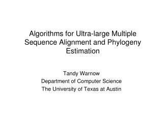
Experimental design • Dataset: 10 real datasets ranging from 1127 to 13921 sequences (DNA and rRNA) • Methods studied: • Recursive-Iterative-DCM3 (Rec-I-DCM3) with 1/4th and 1/8th subset sizes • TNT (combination of simulated annealing, divide-and-conquer, and genetic algorithms) • Five runs of each method: • Rec-I-DCM3: each run for 168 hours (1 week) • TNT: each run for 336 hours (2 weeks)
Results • Performance as a function of time on dataset of 13921 sequences • Comparison of scores found at 168 hours • Rec-I-DCM3 speedup over TNT
5 to 60 minutes on 13921 sequences All three methods are well above best score in the first hour.
1 to 24 hours on 13921 sequences Rec-I-DCM3 scores improve faster than TNT
1 to 336 hours on 13921 sequences • Rapid improvement for both the methods in first 24 hours. • Rec-I-DCM3 continues to improve faster than TNT thereafter.
1 to 336 hours on 13921 sequenceswith all five runs plotted • Plot of all five runs of each method show statistically sound results. • Similar behavior on all datasets.
Average percent above the best known score found to date on each dataset 24 hours 168 hours At 168 hours, Rec-I-DCM3 scores improve by half (above optimal) whereas TNT improvement is slow.
(avg Rec-I-DCM3 time/avg TNT time) to reach avg TNT 2week score Average Rec-I-DCM3 scores reach average TNT score 25 times faster on datasets 9, and 10, and 50 times faster on Datasets 6 and 8 than TNT.
Software • Open source DCM3 code available from http://www.cs.njit.edu/usman • See CIPRES (http://www.phylo.org) • Contact Usman Roshan (usman@cs.njit.edu) or Tandy Warnow (tandy@cs.utexas.edu) for more information
Future work • DCM3–ML • Biological discoveries from large dataset analysis • Optimal subset size
Acknowledgements This work was done in collaboration with • Tandy Warnow (UT Austin and Radcliffe) • Bernard Moret (UNM) • Tiffani Williams (UNM) Thanks to • Pablo Goloboff for support on TNT • Dave Swofford (FSU) for support on PAUP* • Robin Gutell (UT Austin) for providing large accurate alignments • Doug Burger (UT Austin) and Steve Keckler (UT Austin) for usage of the SCOUT Pentium and Mastadon Xeon clusters