Download
1 / 46
470 likes | 580 Views
Logic Programming. Chapter 15 Part 2. Breadth-first v Depth-first Search. Suppose a query has compound goals (several propositions must be satisfied) Depth-first searches prove the first goal before looking at the others. Breadth-first works on goals in parallel.

E N D
Logic Programming Chapter 15 Part 2
Breadth-first v Depth-first Search • Suppose a query has compound goals (several propositions must be satisfied) • Depth-first searches prove the first goal before looking at the others. • Breadth-first works on goals in parallel. • Prolog uses the depth-first approach.
Backtracking • When a compound goal is being proved, it may be that a subgoal cannot be shown true. • In that case, Prolog will back up and try to find another solution to a previous subgoal.
A Partial Family Tree Figure 15.3
A Small Family “Tree” Figure 15.4
Processing Queries ?- father(X, sue)Satisfied with the first comparison. X is instantiated with john. ?- mother(sue, X)Satisfied with X = nancy, X = jeff ?- mother(alice, ron)Fails
?- grandparent(Who, ron). Instantiating grandparent rule from query: Grandparent(Who,ron):- parent(Who,X),parent(X,ron). First, find a fact that satisfies parent (Who,X) This entails finding a fact to satisfy eithermother (Who, X) or father(Who, X) First try: mother(mary, sue) (“mother” rule is first) Next, find a fact that satisfies parent(sue, ron) By satisfying either mother(sue, ron) or father(sue, ron)
Prolog Lists • The list is Prolog’s basic data structure • Lists are a series of Prolog terms, separated by commas • Each list element can be a(n) • atom • variable • sublist • etc.
Examples of Lists • The empty list: [ ] • List with embedded list: [girls, [like, boys]] • List with variables: [x, V1, y, V2, [A, B]] • V1, V2, A, and B are variables that may be instantiated with data at a later time. • Multi-type lists: [boy, [1, 2, 3], ran] • [A, _, Z] • The _ means “don’t care” – sometimes referred to as an unbound variable.
Working with Lists • [Head|Tail] notation simplifies processing: • Head represents the first list element, Tail represents everything else. • Head can be any Prolog term (list, variable, atom, predicate, etc.) • If L = [a, b, c] then Head = a and Tail = [b,c] • Tail is always another list. • What is the head of [a]? The tail? • Compare to car and cdr in Lisp, Scheme
The append Function • append is a built-in Prolog function that concatenates two lists. • append(A, B, L)concatenates the lists A and B and returns them as L. • append([my, cat], [is, fat], L). yieldsL = [my, cat, is, fat] • Compare to Scheme function
The Append Function • append(L1, L2, L3): append([], X, X). %base case append([Head|Tail], Y, [Head|Z]) :- append(Tail, Y, Z). • This definition says: • The empty list concatenated with any list (X) returns an unchanged list (X again). • If Tail is concatenated with Y to get Z, then a list one element larger [Head | Tail] can be concatenated with Y to get [Head | Z].
?- Append([english, russian], [spanish], L). H=english, T=[russian], Y=[spanish], L=[english,Z] 1 and Z = [russian, spanish] Append([russian],[spanish], [Z]). H = russian, T=[ ], Y=[spanish], Z=[russian|Z1] 2 Append([ ], [spanish], [Z1]). So Z1= [spanish] X=[spanish], Z1=[spanish] 3 Append([ ], [spanish], [spanish]).
Using append prefix(X, Z) :- append(X, Y, Z). (finds all prefixes of a list Z) suffix(Y, Z) :- append(X, Y, Z). (finds all suffixes of Z)
Recursion/ member • The function returns ‘yes’ or ‘true’ if X is a member of a given list.member(X, [X | _ ]).member(X, [ _ | Y]) :- member(X, Y).
Member(X,Y) • The test for membership succeeds if either: • X is the head of the list [X |_] • X is not the head of the list [_| Y] , but X is a member of the list Y. • Notes: pattern matching governs tests for equality. • Don’t care entries (_) mark parts of a list that aren’t important to the rule.
Naming Lists • Defining a set of lists: a([single]). a([a, b, c]). a([cat, dog, sheep]). • When a query such as a(L), prefix(X, L). Is posed, all three lists will be processed. • Other lists, such as b([red, yellow, green]), would be ignored.
A Sample List Program a([single]). a([a, b, c]). a([cat, dog, sheep]). prefix(X, Z) :- append(X, _, Z). suffix(Y, Z) :- append(_, Y, Z). % To make queries about lists in the database: % suffix(X, [the, cat, is, fat]). % a(L), prefix(X, L).
Sample Output ?- a(L), prefix(X, L). L = [single] X = [] ; L = [single] X = [single] ; L = [a, b, c] X = [] ; L = [a, b, c] X = [a] ; L = [a, b, c] X = [a, b] ; L = [a, b, c] X = [a, b, c] ; L = [cat, dog, sheep] X = [] Based on the program on the previous slide.
Sample Output 35 ?- a(L), append([cat], L, M). L = [single] M = [cat, single] ; L = [a, b, c] M = [cat, a, b, c] ; L = [cat, dog, sheep] M = [cat, cat, dog, sheep] ;
Recursive Factorial Program To see the dynamics of a function call, use the trace function. For example,given the following function: factorial(0, 1). factorial(N, Result):- N > 0, M is N-1, factorial(M, SubRes), Result is N * SubRes. %is ~ assignment
Logic Programming 15.2.2: Practical Aspects 15.3: Example Applications
Using the Trace Function • At the prompt, type “trace.” • Then type the query. • Prolog will show the rules it uses and the instantiation of unbound constants. • Useful for understanding what is happening in a search process, or in a recursive function.
Tracing Output These are temporary variables ?- trace(factorial/2). ?- factorial(4, X). Call: ( 7) factorial(4, _G173) Call: ( 8) factorial(3, _L131) Call: ( 9) factorial(2, _L144) Call: ( 10) factorial(1, _L157) Call: ( 11) factorial(0, _L170) Exit: ( 11) factorial(0, 1) Exit: ( 10) factorial(1, 1) Exit: ( 9) factorial(2, 2) Exit: ( 8) factorial(3, 6) Exit: ( 7) factorial(4, 24) X = 24 These are levels in the search tree
Tracing 2 ?- trace(factorial/2). % factorial/2: [call, redo, exit, fail] true. [debug] 3 ?- factorial(3, Result). T Call: (6) factorial(3, _G521) T Call: (7) factorial(2, _G599) T Call: (8) factorial(1, _G602) T Call: (9) factorial(0, _G605) T Exit: (9) factorial(0, 1) T Exit: (8) factorial(1, 1) T Exit: (7) factorial(2, 2) T Exit: (6) factorial(3, 6) Result = 6 User-entered commands are in red; other output is generated by the Prolog runtime system.
%remove() removes an element from a list. %To Call: remove(a, List, Remainder). % or remove(X, List, Remainder). % First parameter is the removed item, % 2nd parameter is the original list, % third is the final list remove(X, [X|R], R). remove(X, [H|R], [H|S]):- remove(X, R, S).
18 ?- trace. Yes 18 ?- remove(a, [b, d, a, c], R). Call: (7) remove(a, [b, d, a, c], _G545) ? creep Call: (8) remove(a, [d, a, c], _G608) ? creep Call: (9) remove(a, [a, c], _G611) ? creep Exit: (9) remove(a, [a, c], [c]) ? creep Exit: (8) remove(a, [d, a, c], [d, c]) ? creep Exit: (7) remove(a, [b, d, a, c], [b, d, c]) ? creep R = [b, d, c]
Revisiting The Factorial Function Evaluation of clauses is from left to right. Note the use of is to temporarily assign values to M and Result
Simple Arithmetic • Integer “variables” and integer operations are possible, but imperative language “assignment statements” don’t exist.
Sample Program speed(fred, 60). speed(carol, 75). time(fred, 20). time(carol, 21). distance(X, Y) :- speed(X, Speed), time(X, Time), Y is Speed * Time. area_square(S, A) :- A is S * S.
Prolog Operators • is can be used to cause a variable to be temporarily instantiated with a value. • Compare to assignment statements in declarative languages, where variables are permanently assigned values. • The not operator is used to indicate goal failure. For example not(P) is true when P is false.
Arithmetic • Originally, used prefix notation +(7, X) • Modern versions have infix notationX is Y * C + 3. • Qualification: Y and C must be instantiated, as in the Speed program, but X cannot be (It’s not a traditional assignment statement). • X = X + Y is illegal. • X is X + Y is illegal. “Arguments are not sufficiently instantiated”
More About Arithmetic • Example of simple arithmetic, using something similar to Python’s calculator mode (not as part of a program). • ?- X is 3 + 7. • X = 10 • Yes • Arithmetic operators: +, -, *, /, ^ (exponentiation) • Relational operators: <, >, =, =<, >=, \=
The cut & not Operators • The cut (!) is used to control backtracking. • It tells Prolog not to retry the series of goals that precede the cut symbol (if the goals have succeeded once). • Reasons: Faster execution, saves memory • Not(P) will succeed when P fails. • In some places it can replace the ! Operator.
Example: Revised Factorial factorial(N, 1):- N < 1, !. factorial(N, Result):- M is N – 1, factorial(M, P), Result is N * P. factorial(N, 1):- N < 1. factorial(N, Result):- not(N < 1), M is N–1, factorial(M, P), Result is N * P.
When Cut Might Be Used(Clocksin & Mellish) • To tell Prolog that it has found the right rule: • “if you get this far, you have picked the correct rule for this goal.” • To tell Prolog to fail a particular goal without trying other solutions: • “if you get to here, you should stop trying to satisfy the goal.” • “if you get to here, you have found the only solution to this problem and there is no point in ever looking for alternatives.”
Assert - Adding Facts • ?- assert(mother(jane, joe)).adds another fact to the database. • More sophisticated: assert can be embedded in a function definition so new facts and rules can be added to the database in real time. • Useful for learning programs, for example.
Symbolic Differentiation Rules Figure 15.9
Prolog Symbolic Differentiator Figure 15.10
Search Tree for the Query d(x, 2*x+1, Ans) Figure 15.11
Executing a Prolog Program • Create a file containing facts and rules; e.g., familytree.pl • Follow instructions in handout, which will be available Wednesday.
SWIplEdit “compile” error • If SWI-Prolog finds an error in the .pl file it will give a message such asERROR: c:/temp/prologprogs/remove.pl:18:0: Syntax error: Illegal start of term(18 is the line number)
Runtime Error Message • The function samelength was called with one parameter when it needed 2:21 ?- samelength(X).ERROR:Undefined procedure: samelength/1ERROR:However, there are definitions for: samelength/2
Runtime Errors • Here, the error is an error of omission:22 ?- samelength([a, b, c,],[a, b]) |Queries must end with a period. If you hit enter without typing a period SWIpl just thinks you aren’t through.
Using SWI Prolog • If there is an error that you can’t figure out (for example you don’t get any answers, you don’t get a prompt, typing a semicolon doesn’t help) try “interrupt” under the Run button. • If changes are made to the program, don’t forget to save the file and “consult” again.