Download
1 / 27
270 likes | 423 Views
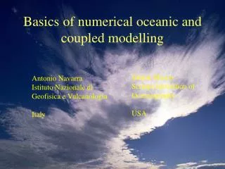
Basics of numerical coupled modelling. Antonio Navarra Istituto Nazionale di Geofisica e Vulcanologia Italy. Sea Ice. Precipitation. Evaporation. Run-off. Oceans. The Climate System. Atmosphere. Biosphere. Soil Moisture. Coupled Phenomena.

E N D
Basicsof numerical coupled modelling Antonio Navarra Istituto Nazionale di Geofisica e Vulcanologia Italy
Sea Ice Precipitation Evaporation Run-off Oceans The Climate System Atmosphere Biosphere Soil Moisture
Coupled Phenomena Why is there a need for considering coupled models ? There are at least two major reasons why it is clear that realistic description of climate cannot be done without considering the atmosphere and ocean at the same time Teleconnections The interactions between atmosphere and oceans in the tropics dominate the variability at interannual scales. The Sea Surface Temperature affects the atmosphere generating giant patterns that extend over the planet Thermohaline Circulation The deep oceanic circulations is driven by fluxes of heat and fresh water that change temperature and salinity of the water. Dense water (cold and saline) sink deep down creating a worldwide circulation as light water (fresh and warm) upwells through the world ocean, affecting the global sea surface temperatures, which in turn change the dominant mode of climate variability through the teleconnections.
Teleconnections PNA NAO PNA North Atlantic Oscillation PNA Monsoon PNA Sahel Nordeste SST SST The interactions between atmosphere and oceans in the tropics dominate the variability at interannual scales. The main player is the variability in the equatorial Pacific. Wavetrains of anomaly stem from the region into the mid-latitudes, as the Pacific North American Pattern (PNA). The tropics are connected through the Pacific SST influence on the Indian Ocean SST and the monsoon, Sahel and Nordeste precipitation. It has been proposed that in certain years the circle is closed and and a full chain of teleconnections goes all around the tropics. Also shown is the North Atlantic Oscillation a major mode of variability in the Euro_atlantic sector whose coupled nature is still under investigation.
Thermohaline Circulation The interactions between atmosphere and ocean in the high latitudes drive the long term circulation of the deep ocean. Cold, dense water sinks int he north Atlantic and in the Antarctica and fills the ocean basins before reemerging as warm surface waters. Based on a CLIVAR transparency Model studies have shown that other circulation are possible with sinking taking place in the North Pacific as well. We do not know if this possibility has ever been realized during the history of the planet.
Numerical Models The only hope we have to be able to understand and possibly predict some of these changes is to use numerical models to investigate the dynamics of atmosphere-ocean dynamics. Atmospheric and ocean numerical models can be put together (coupled) and numerically integrated for hundreds or thousands of years, depending on the realism of the models involved
Solar Radiation Earth Radiation Wind Radiation TRANSPORT TRASPORTO PRESSIONE EMISSION COOLING REFLECTION EMISSION ABSORPTION HEATING Wind Stress Water Vapor Temperature Laten Heat Sensible Heat RAIN EVAPORATION Numerical Models:Atmosphere Oceans -- Soil -- Cyosphere -- Biosphere
Salinity Temperature Laten Heat Flux TRANSPORT Currents Numerical Models:Oceans Atmospheric radiation Atmosphere Solar Radiation Sensible Heat EVAPORATION RAIN TRANSPORT Density Wind Stress
Discretization Methods The atmosphere and the ocean are divided in computational cells: (Temperature, Wind, Rain, Sea Ice, SST, Salinity, … ) both horizontally and vertically. The dimensions of the cell are usually not the same in the atmosphere and ocean component because of the different dynamics. Dimension of the cell (resolution) 200-300 km
Numerical Models:Coupling Atmosphere Surface Temperature Wind Stress Precipitation Solar Radiation Atmospheric Radiation Air Temperature COUPLER: (1) Interpolate from the atmospheric grid to the ocean grid and viceversa. (2) Compute fluxes Wind Stress Fresh Water Flux Sea Surface Temperature Sensible Heat Flux Latent Heat Flux Oceans -- Sea Ice
Very Large Compiuters are needed Project of the Earth Simulator Computer (Japan) : objective, a global coupled model with 5km resolution
Dt Dt Dt Dt Dt Dt Dt Dt Coupling Coupling Coupling Coupling Coupling Coupling Coupling Coupling Experimental Strategy (1) The main problem is how to synchronize the time evolution of the atmosphere with the evolution of the ocean. The most natural choice is to have a complete synchronization (synchronous coupling): Atmosphere Ocean This choice would require to have similar time steps for both models, for instance 30min for the atmospheric model and 2 hours for the ocean model. Computationally very expensive
Coupling Coupling Coupling Coupling Coupling Coupling Coupling Experimental Strategy (2) Another possibility is to exploit the different time scales using the fact that the ocean changes much more slowly than the atmosphere (asynchronous coupling): Atmosphere Dt Dt Integrate for a very long time Integrate for a very long time Ocean This choice save computational time at the expense of accuracy, but for very long simulations (thousands of years) may be the only choice.
Start of integration Coupling Coupling Coupling Coupling Coupling Coupling Coupling Spin-up the ocean with observed atmospheric forcing Start of integration Initialization Robust Diagnostic Integrate the coupled model for a period, e.g. two years, but impose observed surface temperature and salinity Spin-up But sometimes the models are simply started from climatological conditions or, in the case of climate change experiments, the procedure may become much more sophisticated to account for effects from soil and ice.
Balancing the simulations 0 100 200 Years of Simulations Coupled model are much more sensitive than either ocean or atmosphere model alone. There no constraints imposed, as the SST for the atmospheric simulations or the surface winds for the ocean, that can help in guiding the model toward a realistic climate state. The only forcing is given by the external solar radiation and the model must be capable of realizing its own balanced climate state. The model drift from the initial condition as it slowly reaches for its own equilibrium, if the model is realistic the final equilibrium will be very similar to the what we think is the present Earth climate, if the initial condition is well balanced the drift will be small and smooth.
What coupled models can do The first coupled models had large drifts to an unrealistic climate state. It was then proposed to include a correction to partially correct for the poor fluxes that were exchanged between the models. This correction, known as “flux-adjustment” allowed early experiments, but is becoming less necessary in modern models. The following slides will show some of the results from an integration of a coupled model, developed at our institution in collaboration with LODYC in Paris, within the context of a project sponsored by the European Union, SINTEX. The results are however pretty typical of the behaviour of coupled models.
The SINTEX coupled model Coupler OASIS Atmosphere ECHAM-4 Ocean OPA ECHAM-4: Max-Planxk -Institute, Hamburg Roeckner et al., 1996) Global Spectral T30 (3.75 x 3.75 deg) 19 Vertical levels OPA 8.1: LODYC, Paris, Madec et al., 1998) Global 2 deg longitude 0.5 - 2 deg latitude 31 Vertical Levels Climatological Sea Ice Coupling every 3 Hours No Flux Adjustment
Precipitation Coupled models can reproduce precipitation pretty well on a global scale, including the tropical ITCZ and monsoon circulation, but the pattern follow too much the seasonal oscillation of the sun The rain is too much concentrated in the summer hemisphere and the South Pacific Convergence Zone does not have the right shape
Sea Surface Temperature Observations Coupled models can reproduce the over-all pattern, but they tend to be warmer than observations in the eastern oceans and colder in the western portions of the oceans Model Marine Temperature in the model are too narrowly confined to the equator, the observations are wider
Southern Oscillation Coupled models can reproduce the strong coupling between Sea Level Pressure and Sea Surface Temperature as it is shown in this 200 years time series of the Southern Oscillation Index (SOI) and of the SST in the NINO3 area from a simulation. The anticorrelation is pretty clear and the model display a realistic interannual variability
Teleconnections Correlations between the Sea Level Pressure in Darwin and global SLP in the coupled model. The correlations are very realistic Correlations between the Sea Level Pressure in Darwin and global SST in the coupled model. Also in this case the basic teleconnections are there, but the quality is barely satisfactory.
Observations Teleconnections Correlations between the Sea Surface Temperature in the equatorial Pacific (NINO3) and global SST. Results from observations and two 200 years simulations of coupled model are shown, at lower resolution and at a higher resolution . The models reproduce global patterns, but the propagation of the teleconnections into the midlatitude is still poorly represented. Low Resolution High Resolution
Variability (I) Empirical Orthogonal Patterns from coupled models, atmospheric-only models and observations. It is here shown the first EOF for Winter (JFM) Z500 . The models, especially the high resolution coupled model, shows a good resemblance with observations, indicating that the modes of variability of the model are close to the real one. Atmospheric Model Low Resolution Observations Coupled Model Low Resolution Coupled Model High Resolution
Variability (II) Empirical Orthogonal Patterns from coupled models, atmospheric-only models and observations. It is here shown the second EOF for Winter (JFM) Z500 . This is interesting to show that aldo the higher order modes are captured and that the partition of variance between the modes is also realistic. Atmospheric Model Low Resolution Observations Coupled Model Low Resolution Coupled Model High Resolution
Books G. Philander, El Nino, La Nina and the Southern Oscillation, Academic Press A complete monography on the most important coupled phenomenon Washington and Parker, 3-D climate modeling, Academic Press A comprehensive treatment of the numerical techniques used in coupled models Peixoto and Oort, The Physics of climate, AIP Press The climate system at work, a compendium of what the observations are telling us. A. Navarra (ed.), Beyond El Nino, Springer Verlag A recent collection of results from several important modeling groups, useful to have more informations on the performance of coupled models
Web Sites • www.clivar.com • Site of the international CLIVAR program and of the Coupled Model Intercomparison Project (CMIP) • www.dkrz.de • Center of Climate Research, Hamburg, Germany • www.gfdl.gov • Geophysical Fluid Dynamics Laboratory, NOAA, USA • www.noaa.gov • The extensive site put together by NOAA, USA
Conclusion Really, there should be no conclusion. We have only started to understand the behaviour of coupled models and there is still a long way to go. Open problem involved the regulatory mechanisms of variability at longer and longer time scales and the a proper treatment of ice and land processes. Maybe we should follow the following advice: