Download
1 / 22
220 likes | 350 Views
Background Subtraction and Likelihood Method of Analysis: First Attempt. Jose Benitez 6/26/2006. Part I: Background Subtraction. Properties of background:

E N D
Background Subtraction and Likelihood Method of Analysis:First Attempt Jose Benitez 6/26/2006
Part I: Background Subtraction Properties of background: • Hits on non ring pads, where they are not expected, are seen clearly seen in slot 4. These hits create tails on the Cherenkov angle distribution and make the resolution worse. • The time distribution of these hits is like that of Cherenkov photons hence we cannot remove them with a time cut. • The amount of these hits does not grow with photon path length.
Use last property to perform background subtraction: Call this the signal. Direct Photons Indirect Photons Call this the background. beam position 1
Now we should fit accordingly: Beam Position1: Direct Indirect s=11.4mrad s=10.8mrad • Double Gaussian fit. • 3K events used from Run12. • “Bad” MCP pad columns cut out. Important: Background Gaussian must be fixed. • Background Parameters: • Sigma = 30mrad • Mean = 825mrad • Norm = 220
BABAR 9.6mrad ThetaC resolution as function of photon path length after background removal: 2-3 mrad growth with path length has been removed! Conclusion: Background subtraction is necessary for our data.
Part 2: Likelihood method of analysis which incorporates the TOP measurement. Note: Rather than trying to determine a correction to the measured theta it is more logical to measure beta, as will be seen from this method, when both theta and TOP are known for each photon. Step 0: Determine the beta resolution BABAR has from it’s thetaC resolution in order to have a reference to compare to. Step 1: Construct a PDF which describes our data. Step 2: Determine the parameters of the PDF. Step 3: Use the PDF to determine beta for each photon detected. Step 4: Fit the beta distribution to determine our resolution; background subtraction will be used.
Step 0: BABAR beta resolution <l>=410nm <n>=1.469 s=10.4x10⁻³ s=9.6mrad
Step1: Construction of a PDF Physics: Known properties of Cherenkov radiation: • Distribution of photons: Where l is restricted to the range where bn(l) > 1, and b is the speed of the particle which produced the radiation in a medium with index of refraction n(l) . • Correlation of wavelength with theta is exact: The number of photons emitted also depends on q, hence Cherenkov radiation is described by a 2D distribution N(q,l). What is the functional form of this 2D distribution?
Since the correlation of theta with lambda is exact the 2D distribution must be the following: • This relation now combines the previous two equations into one. • There exists a more rigorous way of deriving it. • The delta function confines the probability to a very narrow region/curve of the theta-lambda plane defined by the Cherenkov equation in order to retain the exact correlation. • The factor of bn is there because we must require that Do the math!
Measurement: • N(q,l) is the PDF for an ideal detector which could measure both theta and lambda with no error and with perfect (l independent) efficiency. • For a detector which measures theta and lambda with gaussian errors (sqand sl) and has a l dependent efficiency the PDF can be constructed by convolution with Gaussians and multiplication by the known efficiency e(l) :
We must determine the effciency distribution: • Normalization is not important. • Shape does not change drastically • use same distribution for all photons Limits on wavelength integral: lmin=3000A lmax=6500A Double Gauss Fit
Is the Theta error Gaussian? • Our data does not have a nice Gaussian distribution in theta. I believe this has to do with non-uniform illumination plus insufficient coverage. • Consider toy model for our measurement setup: Non-Uniform illumination : Uniform illumination: Pixelated Distribution Single ring with 5mrad width. Many rings with 5mrad width. Error on Theta will be Gaussian. Dq Gaussian Distribution Dq
Problem: Unfortunately we cannot use this PDF because of the method we use to measure lambda: When the resolution in ng becomes bad there are too many measurements which cannot be converted into a lambda because the map between lambda and ng saturates at about ng=1.44; any measurements of ng below this value do not have a corresponding value of lambda. Furthermore the error on lambda is by far not Gaussian. Group index vs. wavelength Beam Position 1 Direct Photons
Polynomial Fit l(ng)=ng-1 • However this does not pose a real problem in this likelihood method because we can rewrite the PDF in terms of the photon speed v since there is a one-to-one map between v and lambda: • Note we have acquired a new factor dl/dv from the Jacobian of the transformation. • Finally, the PDF becomes: Limits on velocity integral: nmin=v(lmin) nmax=v(lmax)
Step 2: Determination of the PDF parameters: • Since we measure the speed of the photons as and the errors on L and T appear to be Gaussian it follows that the error on v is Guassian. So we have solved both of our previous problems by working on the q-v plane. • We must determine our resolutions sqand sn by projecting the PDF onto the theta and v axes and fitting it to our data: • These fits are done by trial and error so they are not optimized, however our beta resolution will turn out to be almost independent of these parameters. These parameters are likely to important when doing PID Projections of the PDF: sq~9mrad , sn=9x10⁻³ Data is from Beam Position 1 Indirect Photons
Check PDF at perfect Theta and V resolution PDF with parameters : b=1, sq~.5mrad , sn =.5x10-3 Theta Projection RMS~3.7mrad q (rad) Velocity Projection RMS~8.5x10⁻³ v/c
Measurement of velocity resolution as a function of photon path length: Growth is due to the increasing relative error in time measurement, the saturation comes from the constant relative error in the path length. sL/L ~ 1.3% sT ~ 285ps • Used new pad angle assignments and slot dependent time epsilons from Joe. There is some help from the epsilons but it is not significant. • There is significant help from using total photon path length rather than just the bar path length.
2D Plot of the PDF Assuming the following parameters: sq~9mrad b=1 sn=9x10⁻³ Data From Beam Position 1 Indirect photons PDF(q, v) q q n n PDF follows curve which is determined by Cherenkov Equation
Step3: Determination of beta for each photon using the PDF. • Each photon is described by the angle q and velocity v. • To find the beta which produced this photon we scan beta from some minimum to some maximum value and feed our two measurements into the PDF for each beta. The PDF assigns a probability to each value of beta and we take the beta with the largest probability. Example: Using the PDF these lines are smeared and Measurement 2 is not cut out. Measurement 1 b=.97 .. q (rad) b=1.04 b=1.03 b=1.02 Measurement 2 b=? b=1.01 b=1 b=.99 b=.98 b=.97 b=.96 .. n Terminal point v~.68
Step4: Fit beta distribution. • Apply Background Subtraction. Beam Position 1 Indirect photons. sb=11.4x10⁻³ sb=10.9x10⁻³ Background Gaussian must be fixed. • Background Parameters: • Sigma = 30x10-3 • Mean = 1.004 • Norm = 250 • Double Gaussian fit. • 3K events used from Run12. • “Bad” MCP pad columns cut out.
Beta Resolution as a function of photon path length: BABAR 10.4x10⁻³
Conclusions • Background subtraction is very powerful. If we would let the background Gaussian be bigger the signal resolution would be even better possibly as good as BABAR. • A PDF which describes our data has been constructed. The only problem is that our data does not have a Gaussian error; however when the detector plane is uniformly illuminated the error will become Gaussian. • Our current resolution on the photon velocity is higher than expected for a TOP resolution of 100ps and a path length resolution of 1%. The saturation in the v resolution appears to indicate that the path length resolution is actually worse. • The main advantage of the likelihood method is that it provides a function into which we can feed our measurements without having to cut out any photons independent of the resolution in v (or ng). • A clear chromatic correction is seen when we use the likelihood method.