Download
1 / 82
830 likes | 984 Views
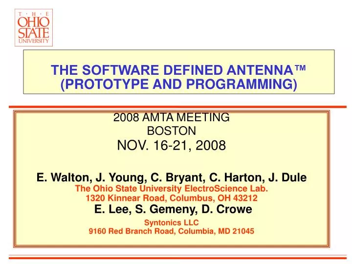
2008 AMTA MEETING BOSTON NOV. 16-21, 2008 E. Walton, J. Young, C. Bryant, C. Harton, J. Dule The Ohio State University ElectroScience Lab. 1320 Kinnear Road, Columbus, OH 43212 E. Lee, S. Gemeny, D. Crowe Syntonics LLC 9160 Red Branch Road, Columbia, MD 21045.

E N D
2008 AMTA MEETING BOSTON NOV. 16-21, 2008 E. Walton, J. Young, C. Bryant, C. Harton, J. DuleThe Ohio State University ElectroScience Lab.1320 Kinnear Road, Columbus, OH 43212 E. Lee, S. Gemeny, D. Crowe Syntonics LLC9160 Red Branch Road, Columbia, MD 21045 THE SOFTWARE DEFINED ANTENNA™ (PROTOTYPE AND PROGRAMMING)
RECONFIGURABLE ANTENNA GOALS(WE ARE SERIOUS ABOUT THIS; prototype in 3 months) • Freqs: • 200 MHz to 18 GHz • (ya gotta be kidding ) • Gain: >30dBi goal • Polarization Goals: • V, H, RH Circular, LH Circular, Slant • I.E. “any” • Mechanical • Mechanically strong • Conformal • Speed • Complete reconfiguration in < 1 ms
Research Highlights • Analytic highlights: • Use HFSS (by Ansoft Corp) to model Cap-on-Post concept • Model the transmission lines based on finite dielectric • Good agreement between experimental testing and HFSS models • Experimental highlights: • We created effective pixel-based microstrip transmission lines • Pixel-based t-lines were shown to be reconfigurable and effective • We successfully demonstrated pixel based t-lines feeding patch antennas • single patch • two element steered beam array • Therefore, PARCA antenna concept is feasible! • Pixel size ≤ l/10 continues to seem appropriate • Determines high frequency limit • Precision inter-pixel gaps are critical to performance • Determines low frequency cut-off • Triangular, square, and hexagonal pixels are candidates
w εr H WIDTH VS. HEIGHT THAT WILL YIELD A 50 OHM TRANSMISSION LINE. From the literature: We note that a 6/32 nut is7 mm across (flat to flat or “average” and 3 mm thick for a W/H ratio of 2.3. It can be supported on a nylon 6/32 nut (nylon εr is 4). Such a transmission line will be very close to 50 ohms. Much early work done with this “standard” test pixel. HFSS model
Example HFSS geometries WE HAVE DONE SEVERAL STUDIES BASED ON THIS MODEL
TRANSMISSION LINES EARLY EXPERIMENTAL TESTING EARLY TEST LINE PATH 2 (REFERENCE) PATH 1 (2-WIDE NUT ROW)
PRELIMINARY TRANSMISSION DATA • Thru = coax adapter • Barcover = solid metal strip • 2wide = hex geometry with two hex nuts wide (see photo) • 1gap = T-Line with a gap of a pair of hex nuts • Allgone = all of the T Line removed. The rolloff is caused by the characteristics of the coax lines used to feed the structure.
VARIOUS SIZES OF PATCH ANTENNAS WERE TESTED (IMPEDANCE (S11) AND GAIN (S21) PIXEL-BASED PATCH ANTENNAS ARE PRACTICAL EXAMPLE: 6X13 NUT PATCH ANTENNA
analytic modeling • Modeling allows us to extend simulations to beyond what is possible in these feasibility experiments. • Different dielectrics (including variations in the loss tangent) • Different pixel geometries • Different spacing between pixels • Antenna array modeling
Technical approach to modeling Used HFSS by Ansoft Corp. • 3D electromagnetic field simulation • 3D full-wave Finite Element Method (FEM) • extract parasitic parameters (S, Y, Z) • visualize 3D electromagnetic fields (near- and far-field) • generate broadband SPICE models • optimize design performance. • HFSS evaluates • transmission path losses • reflection loss due to impedance mismatches • parasitic coupling • Radiation
HFSS MODEL EXAMPLE • Nut over washer • Nylon washer with hole • Measured dielectric is 2.0 for washer • This assumes there is no hole, • i.e. measures effective dielectric • Models will use a washer w/o internal hole
Varying inter-pixel gaps, pixel holes vs. solid, pixel shapes, patch feed schemes
1x34 TL CRES/Nylon w/ Brass feed 0 -5 Sim (0.03 mm) -10 ) B -15 measured d ( 1 -20 2 S Sim (0.2 mm) -25 Simulated at s=0.031mm -30 Simulated at s=0.2mm measured -35 1000 2000 3000 4000 5000 6000 7000 8000 9000 10000 frequency (MHz) S21 COMPARISON TO MEASUREMENTS DISCRETE SWEEP WE LEARN THAT OUR MEASUREMENTS CORRESPOND TO 0.2 mm SPACING.
0 0 -5 -5 -10 -10 -15 -15 -20 -20 -25 -25 -30 -30 -35 -35 0 500 1000 1500 2000 2500 0 500 1000 1500 2000 2500 HFSS study of different geometries and separations 1x10 TL hex nuts, s = 0.1 mm 1x10 TL hex nuts, s = 0.005 mm hex nuts, s = 0.0025 mm square nuts, s = 0.1 mm square nuts, s = 0.005 mm square nuts, s = 0.0025 mm hex nuts, s = 0.1 mm squares, s = 0.1 mm hex nuts, s = 0.005 mm squares, s = 0.005 mm hex nuts, s = 0.0025 mm squares, s = 0.0025 mm square nuts, s = 0.1 mm S11 S21 square nuts, s = 0.005 mm square nuts, s = 0.0025 mm squares, s = 0.1 mm squares, s = 0.005 mm squares, s = 0.0025 mm NOTE: LOW FREQ. EXTENDS TO 10 MHZ NOTE: LOW FREQ. EXTENDS TO 10 MHZ frequency (MHz) frequency (MHz) • LOW FREQ. PERFORMANCE: • SQUARE NUTS ARE BETTER THAN HEX • THE HOLE IN THE NUT MAKES LITTLE DIFFERENCE
S parameters for smaller separation transmission line • S = 0.005 mm • 35 min • S = 0.025 mm • 92 min • S = 0.100 mm • 43 min • Cutoff frequency decreases as separation between nuts is reduced “nuts” @ stainless steel
Stub tuning for a 5x5 patch 21 tuned This was eyeballed and did not turn out as good as I had hoped. I will do another version where I calculate the stub tuning more precisely. original
d=1,l=1:5 22 STUB TUNING CONCEPT d l
SIMULATION STUDY – QUICK IMPRESSIONS • Separation between pixels • Smaller is much better • Results in a lower cutoff frequency • Allows operation at the lower frequencies that we have been reaching for • Multi-width TL • Single width transmission line is closest to 50 ohms. • Switch from capacitive to inductive • Square pixels • Switch from capacitive to inductive • Lower cutoff freq.
[1] Conclusions drawn from simulations • Inter-pixel gap dimension sets low-frequency cut-off • High frequency: 18 MHz is feasible • Low frequency: 100 MHz seems feasible, 50 MHz may be feasible (but challenging) • Jagged edge formed by hex pixels does not seen to effect performance • Relative surface area of adjacent pixel faces effects performance at low frequencies • E.g., square pixels with same width as hexagon pixels have faces with more surface area
[2] Conclusions drawn from simulations • Discrete versus interpolated scans in HFSS • Interpolated scans — which calculate much faster — are adequate for preliminary design calculations • Detail is lost but general trends are calculated adequately • Discrete scans of large designs will require more computer horsepower • Simulation of feed point deserves careful study • Feed geometry effects S11, S21 performance • We need to better understand how the software is treating this important detail
Dielectric Breakdown at High PowerMay be a problem 26 1st gap Gap comparisons Vs. E-Field Intensity 2nd gap
Phase I experimental results • Technical approach to experiments • Test setups • Transmission line experiments • Patch antenna experiments • Conclusions drawn from experiments
Technical approach to experiments • Fixture • Feed structures through (finite) copper ground planes • S11, S21, and pattern measurements taken indoors in laboratory • Pixels • 6-32 nuts in steel, CRES • Some nuts filled with 6-32 screw • Dielectric • Nylon washers, nylon nuts, Plexiglas strips, glass strips • Patch antennas • Hand-formed, inter-pixel gaps controlled by roughness of nuts • Transmission lines • Hand-formed, inter-pixel gaps controlled by roughness of nuts • Various feed point designs
OPEN ENDED LENGTH OF TRANSMISSION LINE (A STUDY OF LOSS EFFECTS) S11 RADIATION ZONE STANDING WAVE ZONE 5 nuts7 nuts11 nuts 2-HIGH LAYER OF HEX NUTS OVER NYLON
TRANSMISSION LINE DIRECT COMPARISON “With cover” is a surrogate for very small gaps. 10 dB loss Good agreement with EYL’s theoretical SEPT 27, 2006 DATA
INTRINSIC IMPEDANCE STUDY • THESE RESULTS ARE INFLUENCED BY RADIATION FROM THE LINE AND THE FEED POINT CONNECTOR • RADIATION FROM THE LINE LOOKS LIKE LINE LOSS • THE BEST BEHAVIOR HERE IS THE 2-NUT WIDE FILLED HOLE EXAMPLE. (But that is only if 50 ohms is considered desirable.) (50 ohms is an arbitrary number in any case.) • MUCH OF THE IMPEDANCE IS SOMEWHAT CLOSE TO 50 OHMS • BUT THE REACTIVE LINE IMPEDANCE VARIES FROM CAPACITIVE TO INDUCTIVE
PUSH FREQUENCY LOWER TRANSMISSION LINE MEASUREMENTS EXTENSION TO LOWER FREQUENCIES GEOMETRY
stack em' STACK NUTS 1 – 2- 3 HIGH NOTE MOVE TO LOWER FREQUENCIES
Rack em' MAKE T-LINES WIDER NOTE COMPARISON TO “BRIDGE” WASHERS
T-LINE LOW FREQUENCY STUDY GEOMETRY CONCLUSIONS • STACKING THE NUTS HIGHER IMPROVES THE LOW FREQ. BEHAVIOR • WIDER TRANSMISSION LINE IMPROVES THE LOW FREQ. BEHAVIOR (THIS IS THE MOST EFFECTIVE LOW FREQ. CONCEPT.) • THE “BRIDGE” CONCEPT IS USEFUL (BUT NOT PROVEN TO BE AS EFFECTIVE AS THE WIDER T-LINES IN EXTENDING THE LOW FREQ. BEHAVIOR)
TRANSMISSION LINE DIELECTRIC STUDY S21 -- NYLON (εr=4) AND GLASS (εr=6) SUBSTRATES
TRANSMISSION LINE DIELECTRIC STUDY CONCLUSIONS DIELECTRIC STUDY; CONCLUSIONS • CHANGING THE DIEL. CHANGES THE T-LINE IMPEDANCE • BUT SO DOES CHANGING THE WIDTH • HIGHER DIELECTRIC IMPROVES THE LOW FREQUENCY TRANSMISSION COEFFICIENT. • BUT NOT THE HIGH FREQUENCY • INCREASING THE WIDTH OF THE T-LINE ALSO IMPROVES THE LOW FREQUENCY TRANSMISSION COEFFICIENT. • AND THIS CAN BE DONE UNDER COMPUTER CONTROL
ANTENNAS WE CAN CREATE A PIXEL PATCH ANTENNA FOR TESTING
VARIOUS SIZES OF PATCH ANTENNAS WERE TESTED (IMPEDANCE (S11) AND GAIN (S21) EXAMPLE: 6X13 NUT PATCH ANTENNA
ANTENNA TESTING (by a crack team of ESL students) TEST SETUP Lee Das Salisbury SCAN IN AN ARC (>30 INCHES FROM NUT ANTENNA 2-18 HORN 2 NETWORK ANALYZER “GOOD” CABLES 1 ROTATE THE HORN TO OPTIMIZE THE POLARIZATION
INPUT IMPEDANCE TESTING DIFFERENT SIZED ANTENNAS CLASSICAL PATCH EQUATION: 2.12 2.47 2.97 3.71 GHz “FULL LINE” IS A LINE FROM CONNECTOR TO CONNECTOR NOTE STANDING WAVE PATTERNS (BEHAVIOR AS EXPECTED (sort of) )
TESTING OF FEED LINE WITH ANTENNA (DIFFERENT LENGTH FEED LINE) 4 x 9 antenna “FULL LINE” IS A LINE FROM CONNECTOR TO CONNECTOR WE ARE MEAS. S11 FOR THE SAME ANTENNA BUT WITH DIFFERING LENGTH INITIAL TRANS. LINES
OVERVIEW: Plots of Gain vs. Freq. vs. off-boresight angle. For different sized nut antennas 5x11 Horn gain ~ 9 dBi 6x13 7x15 Note the decreasing operational freq. with increasing size as expected
STUB TUNING SEQUENCE (S21) 5 NUTS FROM FEED 7 NUTS FROM FEED 9 NUTS FROM FEED
CONCLUSIONS FROM ANTENNA TUNING TESTS • WE ARE ABLE TO TUNE THE ANTENNA USING IMBEDDED SLOT TECHNIQUES. (removing “A” or “A&B”) (this was also demonstrated previously) • WE ARE ABLE TO TUNE THE ANTENNA USING STUB-TUNING TECHNIQUES • WITH A WELL-TUNED SYSTEM, THE GAIN IS APPROXIMATELY 6 DBi (AS EXPECTED)
SINGLE PATCH OPTIMIZATION TESTS • BUILD A SINGLE PATCH ANTENNA AND MEASURE E & H – PLANE PATTERNS AND IMPEDANCE
SINGLE PATCH GAIN PATTERNS GEOMETRY DEFINITIONS + 60º SIDE-TO-SIDE (H-FIELD CUT) INSTRUMENTATION HORN +60º FRONT-TO-BACK (E-FIELD CUT) -60º -60º
ANTENNA GAIN PERFORMANCE STUDY (SINGLE PATCH ANTENNA 5x11 NUTS - SUMMARY) SIDE-SIDE FULL PATCH - GAIN “A”tuning “AB” tuning FRONT - BACK 3-NUT WIDE T-LINE
s f b s ANTENNA PERFORMANCE STUDY (SINGLE PATCH 5X11 VS 7X15 NUTS “AB” tuning) Side-Side 2.75 – 2.5 GHz 4 – 3.5 GHz Freq. shift and patch size should be in same proportion. 4/3.5 = 1.14 ratio; 2.75/2.5 = 1.1 ratio; size 7/5 = 15/11 =1.4 ratio 3-NUT WIDE T-LINE