Download
1 / 21
210 likes | 319 Views
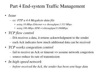
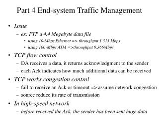
Part 4 End-system Traffic Management. Issue ex: FTP a 4.4 Megabyte data file using 10-Mbps Ethernet => throughput 1.313 Mbps using 100-Mbps ATM =>throughput 0.366Mbps TCP flow control DA receives a data, it returns acknowledgment to the sender

E N D
Part 4 End-system Traffic Management • Issue • ex: FTP a 4.4 Megabyte data file • using 10-Mbps Ethernet => throughput 1.313 Mbps • using 100-Mbps ATM =>throughput 0.366Mbps • TCP flow control • DA receives a data, it returns acknowledgment to the sender • each Ack indicates how much additional data can be received • TCP works congestion control • fail to receive an Ack or timeout => assume network congestion • source reduce its rate of transmission • In high-speed network • before received the Ack, the sender has been sent huge data
Chapter 11 Link-Level Flow and Error Control • Flow Control • limit the amount or rate of data that is sent • Why needs flow control • destination protocol processing may slower than transmitter • limited buffer capacity may fill up • Link-level flow control (physical link) • Network-level flow control (logical connection) • Error Control :to recover from the loss or damage of PDU • involve error detection (based on a frame check sequence ) • PDU retransmission
Link Control Mechanisms • Why we need to segment message into a sequence of frames • receiver buffer size is limited • if incurs error, retransmission overhead is small • fairness on the shared medium • Link-level flow and error control • stop and wait • sliding windows • Go-Back-N • selective reject
Stop and Wait • Sender sends a frame and wait until it receives the Ack sent by the receiver • two types of errors • Tx data error (CRC detection) => no Ack • source station actives a timer when it sends a frame • Ack error => source time out and retransmission • receiver receives duplicate frame • 1-bit sequence number • automatic repeat request (ARQ) • use error detection, timers , acknowledgments, and retransmission
Stop-and-Wait utilization • Fig. 11.4 illustrates the link utilization • assuming no errors, the maximum sending frame rate is 1/Tframe, • the maximum stop-and-wait maximum frame rate is 1/(Tframe + 2Tprop+Tack) • Tprop: the duration between the first bit of frame leaves from source and the first bit of the frame arrives at destination • Tframe: the transmission time for the data frame • Tack: the transmission time for the Ack frame
Sliding-window Techniques • Window size n: destination station buffer capacity • sender is allowed to send n frames without waiting for any Ack • Sequence number: to keep track of which frames have been Ack. • Ack. Frame includes the sequence number of the next frame expected • if ack’s sequence number is 5, it means that frame 1,2,3,4 have been received • Fig. 11.5 and Fig. 11.6 depict the sliding-window process • RR3 means receive ready 3 (equal to Ack3)
Go-back-N ARQ • Most commonly used of the sliding-window • if destination detects a error frame, it sends a REJ frame (reject ack frame) and discard all future incoming frames until the frame in error is correctly received • sender must retransmit the frame in error plus all succeeding frames • three cases for damaged frame :(A: sender, B: receiver) • B detects i-frame error, B sends REJ i. A retransmit i-frame and all subsequent frames • Frame i lost, and receive frame (i+1) (out of order), B sends REJ i, • Frame i loss, and A timeout, A send a RR frame with a P bit of 1, B must be Ack . If A receives the Ack, then retransmit frame i
Two cases for damaged RR • B sends RR(i+1) but loss, but before A timeout for the frame i, A receives RR(i+2) • if A’s timer expires, send an RR with P bit set to 1 and set another timer. If the p-bit timer still timeout, A try again to send RR with p-bit set to 1 and active timer. After maximum number trying, A initiates a reset procedure • Damaged REJ. If a REJ is lost, like A’s timer expires • Fig. 11.7A depicts the go-back-N ARQ • Fig. 11.7B depicts the Selective-reject ARQ
ARQ Performance • Error free stop-and-wait The time to send one frame is T T = Tframe+Tprop+Tproc+Tack+Tprop+Tproc = Tframe + 2 Tprop The throughput S = Tframe/(Tframe+2Tprop) = 1/(1+2a), where a = Tprop/Tframe • Stop-and-wait ARQ with Errors T = Tframe + Timeout + Tframe + 2 Tprop (if one error) = 2(Tframe + 2 Tprop ), if Timeout = 2 Tprop T = Nx (Tframe + 2 Tprop ) Nx is the number of times each frame must be transmittted then the throughput S = Tframe/ Nx(Tframe+2Tprop) = 1/ Nx(1+2a)
With probability to derive Nx Pr(exactly k attempts) = Pr[(K-1) unsuccessful] * Pr(successful) = Pk-1 * (1-P), where P is frame error prob. Therefore, Nx = E[transmissions] = SUMi=1infinit [i*Pr(i transmssions)] = 1/(1-P) Stop and Wait: S = (1-P)/(1+2a) Fig. 11.8 (a) and Fig. 11.8 (b) illustrate the a > 1 and a < 1, separately if ATM cell = 424 bit with 155.52 Mbps physical layer over 106M optical, then the throughput = 1/2445 = 0.0004 if 10Mbps ethernet, frame size = 1000bits, distance range from 100M to 10km, then the throughput in the range of 0.5 to 0.99 Fig. 11.9 shows the performance of stop-and-wait with p = 10-3
Sliding-window ARQ • Error-free sliding-window flow control w: window size, frame transmission time is 1, then a: propagation delay, Fig. 11.10 illustrates the operation case1: W >= 2a+1, the transmit continuously with no pause and normalized throughput is 1.0 case2: W < 2a+1, then during 2a+1 time the sender only sent W, the throughput is W/(2a+1) Fig. 11.11 shows the throughput with different window sizes
Normalized Throughput 1 W ≥ 2a + 1 S = W W < 2a +1 2a + 1