Download
1 / 55
580 likes | 816 Views
Modeling Sedimentary Heterogeneity. Ye Zhang Geology & Geophysics http://faculty.gg.uwyo.edu/yzhang/. Strongly encourage students to also read the conclusions to tie the methods together from the earlier part of the text. .

E N D
Modeling Sedimentary Heterogeneity Ye Zhang Geology & Geophysics http://faculty.gg.uwyo.edu/yzhang/ Strongly encourage students to also read the conclusions to tie the methods together from the earlier part of the text.
Heterogeneity in sedimentary deposits: A review of structure-imitating, process-imitating, and descriptive approachesChristine E. Koltermann & Steven M. GorelickWATER RESOURCES RESEARCH, VOL. 32, NO. 9, PAGES 2617–2658, SEPTEMBER 1996 Statistical Methods (Page 2617~2632) + Conclusion Section
Introduction • Natural sedimentary rocks are heterogeneous (spatially varying) at multiple scales; • Heterogeneity formed as a result of complex geologic processes, e.g., deposition, erosion, diagenesis, structural deformation. • Subsurface heterogeneity is poorly known (most of the subsurface rock is inaccessible)
Sedimentary heterogeneity heterogeneity of hydraulic parameter: porosity & permeability (or, hydraulic conductivity, transmissivity) • Permeability (K) varies over 13 orders of magnitude, whereas porosity (0—1) varies much less. • K heterogeneity controls fluid flow & solute transport in the subsurface K is our focus!
K Heterogeneity controls subsurface fluid flow & solute transport, for example: • groundwater flow; • contaminant migration in groundwater; • oil/gas extraction; • geological waste disposal; • geothermal heat extraction. Solute transport video
CO2 Simulation CO2 migration video
Flow & Transport Modeling • Numerical models are used to simulate subsurface flow & transport processes & make recommendations for management; • Because of the importance of heterogeneity, models need to incorporate K variation; • But, how can heterogeneity be created for modeling, when we have so little data about the subsurface?
Image Creation Structure-imitating, process-imitating, & descriptive methods All approaches can mimic natural heterogeneity over a range of scales & consider geologic information. • Some approaches are strictly spatial; • Some are linked to the time evolution of sedimentation. • Some can be conditioned on measurements.
Structure-imitating methods Constrain the geometry of spatial patterns in sedimentary rocks: correlated random fields, probabilistic rules, and deterministic constraints (from facies relations). Approaches: spatial statistical algorithms & sedimentation pattern-matching.
Process-imitating models • Aquifer model calibration: • Use equations of flow and transport to relate K and porosity to hydraulic and solute information (fluid potential, flow rate, concentration) through history matching. • Geologic process models: • conservation of mass + conservation of momentum + sediment transport equations simulate spatial patterns in grain size distributions.
Descriptive methods Couple geologic observations with facies relations to divide a subsurface reservoirs into zones of characteristic hydraulic properties(e.g., hydrofacies)
To summarize (1996): This talk! More has been done since 1996, including “hybrid” approaches. One approach popular in reservoir modeling is to integrate descriptive (deterministic) & structure-imitating (stochastic) methods
Spatial Statistical Methods • Gaussian methods; • Non-Gaussian methods.
Gaussian Methods • produce images of continuous distributions of K; • The joint multivariate probability density function (pdf) of K is Gaussian; • If actual sample values indicate that K is not normally distributed, then its frequency distribution can be modified by a normal scores transform, before the Gaussian methods are used.
Gaussian Methods • Gaussian methods can incorporate descriptive geologic information in 3 ways: • trends in the geology can be represented; • local values preserved by conditioning; • certain geologic features can be included in the variogram (a spatial correlation function) through statistical anisotropy & nested structures.
Gaussian Methods GEOL 5446 Fall, 2013 • Estimation (finding a “best” map): • Kriging; • Cokriging (including Collocated Cokriging) • Simulations (besides the “best”, evaluate uncertainty around the “best” with alternative realizations) • Nearest neighbor • Turning bands • Fourier transform methods • Fractal methods • LU Decomposition • Sequential Gaussian Simulation (SGS) • Co-Simulation (including Collocated CoSimulation) This Talk
Gaussian Methods --- Ordinary Kriging (OK) OK IDS IDS= Inverse Distance Squared (“Contouring”); OK=Ordinary Kriging (one type of Kriging) gives a single “best” map no alternatives from the best map cannot be used to evaluate uncertainty
SGS Multiple Realizations Realization 1 11 sampled f Realization 2 … Realization 10,000
SGS SGS – Limitation SGS is superior to IDS, but it has trouble delineating connected features IDS True
Gaussian Methods -- “Soft” Data Integration (Collocated CoSimulation)
Non-Gaussian Methods • Some use information from a training image, such as transition frequencies between rock types (e.g., MPS). • Indicator thresholds and variograms can be used to represent spatial structure of extreme values (e.g., indicator kriging or Sequential Indicator Simulation). • Probabilistic or geometric rules governing lithologic geometries can be incorporated. • Most non-Gaussian approaches can consider categorical variables, such as rock type.
Non-Gaussian Methods • Estimation (a single “best” map) • Indicator Kriging; • Indicator Principal components • Simulation (uncertainty around the “best” map) • Sequential Indicator Simulation (SIS) • Object-Based Modeling (Boolean Method; Marked Point Process) • Simulated Annealing • Markov Chains approaches This Talk
Non Gaussian Methods --- SIS Model the Nugget Sandstone in southwestern Wyoming for acid gas disposal from gas fields along the Moxa Arch
Non Gaussian Methods --- SIS • Data used: • Well logs (SP, Sonic, Porosity, Resistivity); • Core measurements; • Cross sections (AA’, BB’, CC’, DD’); • Isopach (one for each geological formation); • DD’ is outside the model domain; it helps us define the structure dip.
Correlating well logs: • Twin Creek Top • Nugget Top • Ankarah Top • Thaynes Top (= Ankarah Bottom)
Petrofacies Modeling with SIS Facies Code 9 facies modeled: “0” clayey sandstone; “1” clay; etc. 3 reservoir zones (in gray color; no sufficient well data for SIS)
Acid Gas Injection End of Injection: 50 years from today End of Monitoring: 3000 years from today
SIS is sensitivity to variogram parameter & statistical anisotropy Same sample data, hand-contouring (deterministic; no uncertainty) Hand contour Hand contour SIS: assume “isotropic” pattern isotropic variogram isotropic SIS simulated pattern, vice versa; SIS (one realization) SIS (one realization)
Non Gaussian Methods --- Object-Based Modeling Geologic information probabilistic rules and geometric constraints object distribution, geometry, direction of elongation, and connectedness
22 12 17 5 Object-Based Modeling: Deepwater Oil Reservoir Outcrop Observations of Facies relations High resolution seismic imaging of the channels at different reservoir depths
Object-Based Modeling of Facies http://faculty.gg.uwyo.edu/yzhang/Publications/SPE_114099.pdf
Porosity & K are then modeled within each facies object Porosity • Each facies has a distinct porosity/K distribution; • Petrophysical modeling is done for faciesby facies. Log10(k)
Once the image(s) are created, how are they used in subsurface modeling?
Estimate f at each unsampled location evaluate its pdf (mean f; uncertainty from mean: sf) Created by collocated cosimulation
Where are the tools? • Many software have been developed for geostatistical modeling, e.g., • GSLIB (free) • Commercial (e.g., Petrel, GoCAD)
Petrel (Schlumberger 2009 Training Manual) SGS generated f conditioned to well data only (e.g., well-log-derived porosity) SGS generated f conditioned to well data & a facies probability cube (higher f are forced into the “channel belt” with a high channel facies probability)
Recent advances • Extract information from sedimentological facies models; • Incorporate qualitative geologic info into random field generators; • Simulate depositional processes; Bottomline: Better understanding of geological variability helps us build better models & make better management decisions.
Story of the “Missing Plume” Engineers first assumed homogenous aquifer with isotropic K streamline perpendicular to head contours plume migrates down hydraulic gradient Install wells to intersect the plume for treatment, but no plume is found along the imaginedflow path! Heterogeneity due to buried “channels” in the aquifer K is anisotropic streamline is different (blue) real plume Plainview
Definitions: • Model: GEOL4444 • Simplified representation of reality; • A mathematical model: a set of PDEs used to describe fluid flow and transport. • Simulation (two definitions of “Simulation”) • Solve the flow and transport model with a computer code (GEOL4030) • Stochastic simulation: image creation using geostatistical techniques (GEOL 5446)
Definitions: • Facies: a rock assemblage of like characteristics, usually reflecting the origin of a rock unit; • Differentiating factors: • lithology lithofacies; • fossil content biofacies, • geophysical log characteristics petrophysical facies • hydraulic property hydrofacies or hydrostratigraphic units (hydrogeology) or flow units (petroleum engineering)
Definitions: Connected high K units form conduits called preferential flow paths. The opposite of a preferential flow path is a flow barrier. When the spatial correlation between two variables disappears beyond a separation distance, that distance is called the correlation range(GEOL 5446). Conditioning: method of image generation exactly reproduces data values at measureddata locations.
Definitions Calibration: parameter values in a mathematical model are adjusted to achieve a best match between observed and simulated values. The volume of a measurement is its support or scale of support. In “upscaling,” values defined on a small support are used to create effective values related to a larger support. “Scale” refers to the extent of the field that is sampled, interpolated, viewed, or simulated.