Download
1 / 33
330 likes | 467 Views
Projects. Registration Home work Latex Team Projects. Term papers/Projects proposals are due on Tuesday 10/23/12 Within a week we will give you an approval to continue with your project along with comments and/or a request to modify/augment/do a different project .

E N D
Projects • Registration • Home work • Latex • Team Projects • Term papers/Projects proposals are due on Tuesday 10/23/12 • Within a week we will give you an approval to continue with your project along with comments and/or a request to modify/augment/do a different project. • Please start thinking and working on the project now; your proposal is limited to 1-2 pages, but needs to include references and, ideally, some of the ideas you have developed in the direction of the project (maybe even some preliminary results). • Any project that has a significant Machine Learning component is good. • You can do experimental work, theoretical work, a combination of both or a critical survey of results in some specialized topic. • The work has to include some reading. Even if you do not do a survey, you must read (at least) two related papers or book chapters and relate your work to it. • Originality is not mandatory but is encouraged. • Try to make it interesting!
Examples • Health Application: Learn access control rules to medical records • Work on making learned hypothesis (e.g., linear threshold functions) more comprehensible (medical domain example) • Develop a People Identifier • Compare Regularization methods: e.g., Winnow vs. L1 Regularization • Large scale clustering of documents + name the cluster • Deep Networks: convert a state of the art NLP program to a deep network, efficient, architecture. • Try to prove something
A Guide • Learning Algorithms • Search: (Stochastic) Gradient Descent with LMS • Decision Trees & Rules • Importance of hypothesis space (representation) • How are we doing? • Quantification in terms of cumulative # of mistakes • More later • Perceptron • How to deal better with large features spaces & sparsity? • Winnow • Variations of Perceptron • Dealing with overfitting • Dual representations & Kernels • Beyond Binary Classification? • Multi-class classification and Structured Prediction • More general way to quantify learning performance (PAC) • New Algorithms (SVM, Boosting) • A new perspective of old algorithms (Perceptron; Gradient Descent)
Quantifying Performance • We want to be able to say something rigorous about the performance of our learning algorithm. • We will concentrate on discussing the number of examples one needs to see before we can say that our learned hypothesis is good.
Learning Conjunctions • There is a hidden (monotone) conjunction the learner (you) is to learn • How many examples are needed to learn it ? How ? • Protocol I: The learner proposes instances as queries to the teacher • Protocol II: The teacher (who knows f) provides training examples • Protocol III: Some random source (e.g., Nature) provides training examples; the Teacher (Nature) provides the labels (f(x))
Learning Conjunctions • Protocol I: The learner proposes instances as queries to the teacher • Since we know we are after a monotone conjunction: • Is x100 in? <(1,1,1…,1,0), ?> f(x)=0 (conclusion: Yes) • Is x99 in? <(1,1,…1,0,1), ?> f(x)=1 (conclusion: No) • Is x1 in ? <(0,1,…1,1,1), ?> f(x)=1 (conclusion: No) • A straight forward algorithm requires n=100 queries, and will produce as a result the hidden conjunction (exactly). What happens here if the conjunction is not known to be monotone? If we know of a positive example, the same algorithm works.
Learning Conjunctions • Protocol II: The teacher (who knows f) provides training examples
Learning Conjunctions • Protocol II: The teacher (who knows f) provides training examples • <(0,1,1,1,1,0,…,0,1), 1>
Learning Conjunctions • Protocol II: The teacher (who knows f) provides training examples • <(0,1,1,1,1,0,…,0,1), 1> (We learned a superset of the good variables)
Learning Conjunctions • Protocol II: The teacher (who knows f) provides training examples • <(0,1,1,1,1,0,…,0,1), 1> (We learned a superset of the good variables) • To show you that all these variables are required…
Learning Conjunctions • Protocol II: The teacher (who knows f) provides training examples • <(0,1,1,1,1,0,…,0,1), 1> (We learned a superset of the good variables) • To show you that all these variables are required… • <(0,0,1,1,1,0,…,0,1), 0> need x2 • <(0,1,0,1,1,0,…,0,1), 0> need x3 • ….. • <(0,1,1,1,1,0,…,0,0), 0> need x100 • A straight forward algorithm requires k = 6 examples to produce the hidden conjunction (exactly). Modeling Teaching Is tricky
Learning Conjunctions • Protocol III: Some random source (e.g., Nature) provides training examples • Teacher (Nature) provides the labels (f(x)) • <(1,1,1,1,1,1,…,1,1), 1> • <(1,1,1,0,0,0,…,0,0), 0> • <(1,1,1,1,1,0,...0,1,1), 1> • <(1,0,1,1,1,0,...0,1,1), 0> • <(1,1,1,1,1,0,...0,0,1), 1> • <(1,0,1,0,0,0,...0,1,1), 0> • <(1,1,1,1,1,1,…,0,1), 1> • <(0,1,0,1,0,0,...0,1,1), 0>
Learning Conjunctions • Protocol III: Some random source (e.g., Nature) provides training examples • Teacher (Nature) provides the labels (f(x)) • Algorithm: Elimination • <(1,1,1,1,1,1,…,1,1), 1> • <(1,1,1,0,0,0,…,0,0), 0> • <(1,1,1,1,1,0,...0,1,1), 1> • <(1,0,1,1,0,0,...0,0,1), 0> • <(1,1,1,1,1,0,...0,0,1), 1> • <(1,0,1,0,0,0,...0,1,1), 0> Final hypothesis: • <(1,1,1,1,1,1,…,0,1), 1> • <(0,1,0,1,0,0,...0,1,1), 0> • With the given data, we only learned an “approximation” to the true concept • Is it good • Performance ? • # of examples ?
Two Directions • Can continue to analyze the probabilistic intuition: • Never saw x1=0 in positive examples, maybe we’ll never see it? • And if we will, it will be with small probability, so the concepts we learn may be pretty good • Good: in terms of performance on future data • PAC framework • Mistake Driven Learning algorithms • Update your hypothesis only when you make mistakes • Good: in terms of how many mistakes you make before you stop, happy with your hypothesis. • Note: not all on-line algorithms are mistake driven, so performance measure could be different. Two Directions
On-Line Learning • Two new learning algorithms (learn a linear function over the feature space) • Perceptron (+ many variations) • Winnow • Issues: • Importance of Representation • Complexity of Learning • Idea of Kernel Based Methods • More about features
Motivation • Consider a learning problem in a very high dimensional space • And assume that the function space is very sparse (every function of interest depends on a small number of attributes.) • Can we develop an algorithm that depends only weakly on the space dimensionality and mostly on the number of relevant attributes ? • How should we represent the hypothesis? Middle Eastern deserts are known for their sweetness
On-Line Learning • Of general interest; simple and intuitive model; • Robot in an assembly line, language learning,… • Important in the case of very large data sets, when the data cannot fit memory – Streaming data • Evaluation: We will try to make the smallest number of mistakes in the long run. • What is the relation to the “real” goal? • Generate a hypothesis that does well on previously unseen data
On-Line Learning • Not the most general setting for on-line learning. • Not the most general metric • (Regret: cumulative loss; Competitive analysis) • Model: • Instance space: X (dimensionality – n) • Target: f: X {0,1}, f C, concept class (parameterized by n) • Protocol: • learner is given x X • learner predicts h(x), and is then given f(x) (feedback) • Performance: learner makes a mistake when h(x)f(x) • number of mistakes algorithm A makes on sequence S of examples, for the target function f. • A is a mistake bound algorithm for the concept class C, if MA(c) is a polynomial in n, the complexity parameter of the target concept. On Line Model
On-Line/Mistake Bound Learning • We could ask: how many mistakes to get to ²-±(PAC) behavior? • Instead, looking for exact learning. (easier to analyze) • No notion of distribution; a worst case model • Memory: get example, update hypothesis, get rid of it (??)
On-Line/Mistake Bound Learning • We could ask: how many mistakes to get to ²-±(PAC) behavior • Instead, looking for exact learning. (easier to analyze) • No notion of distribution; a worst case model • Memory: get example, update hypothesis, get rid of it (??) • Drawbacks: • Too simple • Global behavior: not clear when will the mistakes be made
On-Line/Mistake Bound Learning • We could ask: how many mistakes to get to ²-±(PAC) behavior • Instead, looking for exact learning. (easier to analyze) • No notion of distribution; a worst case model • Memory: get example, update hypothesis, get rid of it (??) • Drawbacks: • Too simple • Global behavior: not clear when will the mistakes be made • Advantages: • Simple • Many issues arise already in this setting • Generic conversion to other learning models • “Equivalent” to PAC for “natural” problems (?)
Generic Mistake Bound Algorithms • Is it clear that we can bound the number of mistakes ? • Let C be a concept class. Learn f ²C • CON: • In the ith stage of the algorithm: • Ciall concepts in C consistent with all i-1 previously seen examples • Choose randomly f 2Ciand use to predict the next example • Clearly, Ci+1µCiand, if a mistake is made on the ith example, then |Ci+1| < |Ci| so progress is made. • The CON algorithm makes at most |C|-1 mistakes • Can we do better ?
The Halving Algorithm • Let C be a concept class. Learn f ²C • Halving: • In the ith stage of the algorithm: • all concepts in C consistent with all i-1 previously seen examples • Given an example consider the value for all and predict by majority.
The Halving Algorithm • Let C be a concept class. Learn f ²C • Halving: • In the ith stage of the algorithm: • all concepts in C consistent with all i-1 previously seen examples • Given an example consider the value for all and predict by majority. • Predict 1 if
The Halving Algorithm • Let C be a concept class. Learn f ²C • Halving: • In the ith stage of the algorithm: • all concepts in C consistent with all i-1 previously seen examples • Given an example consider the value for all and predict by majority. • Predict 1 if • Clearly and if a mistake is made in the ith example, then • The Halving algorithm makes at most log(|C|) mistakes
The Halving Algorithm • Hard to compute • In some cases Halving is optimal (C - class of all Boolean functions) • In general, to be optimal, instead of guessing in accordance with the majority of the valid concepts, we should guess according to the concept group that gives the least number of expected mistakes (even harder to compute)
Learning Disjunctions • There is a hidden disjunction the learner is to learn • The number of disjunctions: • log(|C|) = n
Learning Disjunctions • There is a hidden disjunction the learner is to learn • The number of disjunctions: • log(|C|) = n • The elimination algorithm makes n mistakes
Learning Disjunctions • There is a hidden disjunction the learner is to learn • The number of disjunctions: • log(|C|) = n • The elimination algorithm makes n mistakes • Learn from negative examples; eliminate active literals.
Learning Disjunctions • There is a hidden disjunction the learner is to learn • The number of disjunctions: • log(|C|) = n • The elimination algorithm makes n mistakes • Learn from negative examples; eliminate active literals. • k-disjunctions: • Assume that only k<<n attributes occur in the disjunction
Learning Disjunctions • There is a hidden disjunction the learner is to learn • The number of disjunctions: • log(|C|) = n • The elimination algorithm makes n mistakes • Learn from negative examples; eliminate active literals. • k-disjunctions: • Assume that only k<<n attributes occur in the disjunction
Learning Disjunctions • There is a hidden disjunction the learner is to learn • The number of disjunctions: • log(|C|) = n • The elimination algorithm makes n mistakes • Learn from negative examples; eliminate active literals. • k-disjunctions: • Assume that only k<<n attributes occur in the disjunction • The number of k-disjunctions: • log(|C|) = • Can we learn efficiently with this number of mistakes ? What’s possible?
Representation • Assume that you want to learn disjunctions. Should your hypothesis space be the class of disjunctions? • Theorem: Given a sample on n attributes that is consistent with a disjunctive concept, it is NP-hard to find a pure disjunctive hypothesis that is both consistent with the sample and has the minimum number of attributes. • Same holds for Conjunctions. • Intuition: Reduction to minimum set cover problem. • Given a collection of sets that cover X, define a set of examples so that learning the best disjunction implies a minimal cover. • Consequently, we cannot learn the concept efficiently as a disjunction. • But, we will see that we can do that, if we are willing to learn the concept as a Linear Threshold function. • In a more expressive class, the search for a good hypothesis sometimes becomes combinatorially easier. Importance of Representation