Download
1 / 23
240 likes | 462 Views
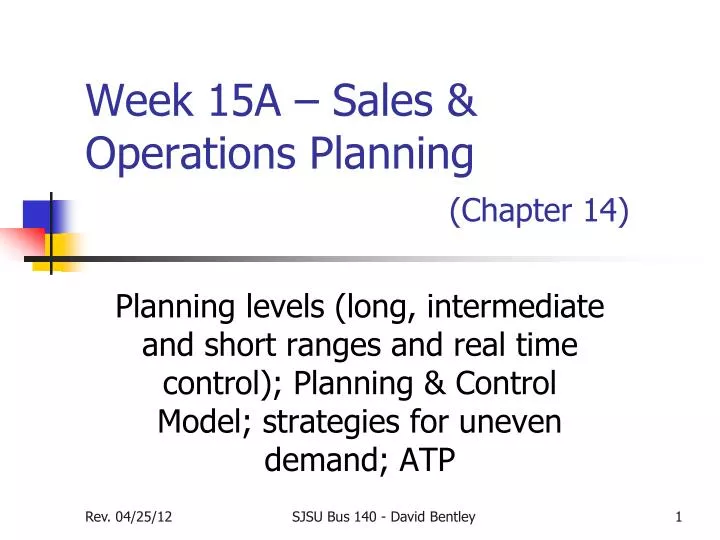
Week 15A – Sales & Operations Planning (Chapter 14). Planning levels (long, intermediate and short ranges and real time control); Planning & Control Model; strategies for uneven demand; ATP. Aggregate Planning Defined. Planning for aggregate demand Total demand stated in some aggregate unit.

E N D
Week 15A – Sales & Operations Planning(Chapter 14) Planning levels (long, intermediate and short ranges and real time control); Planning & ControlModel; strategies for uneven demand; ATP SJSU Bus 140 - David Bentley
Aggregate Planning Defined • Planning for aggregate demand • Total demand stated in some aggregate unit. • Think fruit salad (apples, oranges, berries) • Stated in cups (or some fraction) • Often the unit is $ • May be pounds, square feet, barrels, gallons • Requires eventual disaggregation to specific units SJSU Bus 140 - David Bentley
Planning Levels SJSU Bus 140 - David Bentley
Planning Levels - 1 • Long Range • Horizon: 3-5 years • Intervals (“buckets”): Quarterly and annual • Aggregation: Company, Division, Product Group or Product Line • Consists of: Sales Plan, Operations Plan, Long Range Resource Plan (LRRP) • Supports: Business Plan • Plan and acquire land, buildings, technology SJSU Bus 140 - David Bentley
Planning Levels - 2 • Intermediate Range • Horizon: 18-24 months • Intervals (“buckets”): Monthly and quarterly • Aggregation: Product • Consists of: Demand Forecast, Master Production Schedule (MPS), Rough Cut Capacity Plan (RCCP) • Supports: Sales, Operations, LRR Plans • Hire, develop contracts, add equipment SJSU Bus 140 - David Bentley
Planning Levels - 3 • Short Range • Horizon: 12 months • Intervals (buckets) : Days and weeks • Aggregation: Item (Part) • Consists of: Material Requirements Plan (MRP), Capacity Requirements Plan (CRP) • Supports: Master Production Schedule • Order material, add temps, use overtime SJSU Bus 140 - David Bentley
Planning Levels - 4 • Real Time • Horizon: Now • Intervals (“buckets”): Minutes and days • Aggregation: P.O. line item, Job operation • Consists of: Purchasing system, Production Activity Control (PAC) system (aka Shop Floor Schedule) • Really a control level SJSU Bus 140 - David Bentley
Hierarchical Planning Structure Production Planning Capacity Planning Resource Level Items Sales and Operations Plan Resource requirements plan Product lines or families Plants Master production schedule Rough-cut capacity plan Critical work centers Individual products Material requirements plan Capacity requirements plan All work centers Components Shop floor schedule Input/ output control Manufacturing operations Individual machines SJSU Bus 140 - David Bentley
Disaggregation • Breaking an aggregate plan into more detailed plans • Create Master Production Schedule for Material Requirements Planning • We’ll talk more about disaggregating the plan level-by-level when we come to MRP and MRP II SJSU Bus 140 - David Bentley
Strategies for Uneven Demand • Level Capacity • Steady rate of output • Minimal or no layoffs or hiring • Inventories and/or backlogs • Chase Demand • “Hire and fire” • Varying output rates • Minimal inventory and managed backlog SJSU Bus 140 - David Bentley
Planning Methods • Graphical approaches • Simple to use and understand • Trial-and-error approach • Mathematical approaches • Transportation method, other models • Linear programming approach • See examples which follow SJSU Bus 140 - David Bentley
Pure Strategies Rules specify either pure chase demand or pure level capacity SJSU Bus 140 - David Bentley
Level Production Strategy Level production (50,000 + 120,000 + 150,000 + 80,000) 4 = 100,000 pounds SALES PRODUCTION QUARTER FORECAST PLAN INVENTORY Spring 80,000 100,000 20,000 Summer 50,000 100,000 70,000 Fall 120,000 100,000 50,000 Winter 150,000 100,000 0 400,000 140,000 Cost of Level Production Strategy (400,000 X $2.00) + (140,00 X $.50) = $870,000 SJSU Bus 140 - David Bentley
Level Production with Excel Cost of level production= inventory costs + production costs Input by user=400,000/4 Inventory atend of summer SJSU Bus 140 - David Bentley
Chase Demand Strategy SALES PRODUCTION WORKERS WORKERS WORKERS QUARTER FORECAST PLAN NEEDED HIRED FIRED Spring 80,000 80,000 80 0 20 Summer 50,000 50,000 50 0 30 Fall 120,000 120,000 120 70 0 Winter 150,000 150,000 150 30 0 100 50 Cost of Chase Demand Strategy (400,000 X $2.00) + (100 x $100) + (50 x $500) = $835,000 SJSU Bus 140 - David Bentley
Chase Demand with Excel No. of workershired in fall Workforce requirementscalculated by system Production input by user;production =demand Cost of chasedemand = hiring +firing + production SJSU Bus 140 - David Bentley
Mixed Strategy Combination of Level Capacity and Chase Demand SJSU Bus 140 - David Bentley
Mixed Strategy • Policy examples • “no more than x% of workforce can be laid off in one quarter” • “inventory levels cannot exceed x dollars” • “backorders cannot exceed x units” • May shut down manufacturing during the low demand season and schedule employee vacations during that time SJSU Bus 140 - David Bentley
Mixed Strategy & Linear Programming • LP gives an optimal solution, but demand and costs must be linear SJSU Bus 140 - David Bentley
Mixed Strategy and Excel Target cell;cost of solutiongoes here Solver will put thesolution here When model is complete, Solve Cells where solution appears Click here next Demand Constraint Production Constraint Workforce Constraint SJSU Bus 140 - David Bentley
Strategies for Adjusting Capacity • Overtime and under-time • Increase or decrease working hours • Subcontracting • Let outside companies complete the work • Part-time workers • Hire part-time workers to complete the work • Backordering • Provide the service or product at a later time period SJSU Bus 140 - David Bentley
Strategies for Managing Demand • Shifting demand into other time periods • Incentives • Sales promotions • Advertising campaigns • Offering products or services with counter-cyclical demand patterns • Partnering with suppliers to reduce information distortion along the supply chain SJSU Bus 140 - David Bentley
Available-to-Promise (ATP) • Quantity of items that can be promised to customer • Difference between planned production and customer orders already received SJSU Bus 140 - David Bentley