Download
1 / 46
980 likes | 1.83k Views
Optical Interconnects. Outline. Interconnection Networks Terminology, basics, examples Optical Interconnects Motivation Architecture examples for Data Centers and HPC Building blocks Sum-up - issues. Interconnection Networks: What is an interconnection network?.

E N D
Outline • Interconnection Networks • Terminology, basics, examples • Optical Interconnects • Motivation • Architecture examples for Data Centers and HPC • Building blocks • Sum-up - issues
Interconnection Networks: What is an interconnection network? • Parallel systems need the processors, memory, and switches to be able to communicate with each other • The connections between these elements define the interconnection network
Interconnection Networks: Terminology • Node • Can be either processor, memory, or switch • Link • The data path between two nodes (Bundle of wires that carries a signal) • Neighbor node • Two nodes are neighbors if there is a link between them • Degree • The degree of a node is the number of its neighbors • Message • Unit of transfer for network clients (e.g. cores, memory) • Packet • Unit of transfer for network
Interconnection Networks: Basics • Topology • Specifies way switches are wired • Affects routing, reliability, throughput, latency, building ease • Layout and Packaging Hierarchy • The nodes of a topology are mapped to packaging modules, chips, boards, and chassis, in a physical system • Routing • How does a message get from source to destination • Static or adaptive • Flow control and Switching paradigms • What do we store within the network? • Entire packets, parts of packets, etc? • Circuit switching vs packet switching • Performance • Throughput, latency. Theoretically and via simulations
Interconnection Networks: Topology • Direct topology and indirect topology • In direct topology: every network client has a switch (or router) attached • In indirect topology: some switches do not have processor chips connected to them, they only route • Static topology and dynamic topology
Interconnection Networks: Topology • Examples (Direct topologies): 6-linear array 6-ring 6-ring arranged to use short wires 2D 16-Mesh 2D 16-Torus 3D 8-Cube
Interconnection Networks: Topology • Examples (Indirect topologies): Trees H-layout Fat Trees: Fatter links (really more of them) as you go up 8-node butterfly
Interconnection Networks: Topology • Theoretical topology evaluation metrics: • Bisection width: the minimum number of wires that must be cut when the network is divided into two equal sets of nodes. • Bisection Bandwidth:The collective bandwidth over bisection width • Ideal Throughput: throughput that a topology can carry with perfect flow control (no idle cycles left on the bottleneck channels) and routing (perfect load balancing). Equals the input bandwidth that saturates the bottleneck channel(s) for given traffic pattern. For uniform traffic (bottleneck channels = bisection channels): • Network Diameter • Average Distance (for given traffic pattern). For uniform traffic: • Average zero Load Latency (related to average distance) • Simulations • Throughput, average latency vs offered traffic (fraction of capacity) for different traffic patterns
Topology optimized for Prototype Traffic Patterns Super LU HPC application FFT HPC application • Traffic patterns (locality, message size, inter-arrival times) play an important role • HPC applications exhibit well defined communication patterns (“13 kernels” identified) • Super LU: locality (low degree of connectivity topologies are efficient) • FFT: large, global, point-to-point communication (topologies with good bisection width needed) • DataCenters are multi-tenant environments, various applications, wide variations of requirements (eg for Cloud DCs 75% of traffic remains intra rack). • Hot: Mapreduce – Hadoop application
Interconnection Networks: Layout and Packaging Hierarchy • Blue Gene/L
Interconnection Networks: Layout and Packaging Hierarchy • Layout: important, since it improves the cost performance of the resulting architecture, both by reducing its cost (fewer chips, boards, and assemblies) and by lowering various performance hindrances, such as signal propagation delay, power losses. • Layout area depends on the wiring layers Collinear layout for a hypercube 2-D layout for a hypercube
Interconnection Networks: Layout and Packaging Hierarchy board • Packaging: must take into account board pinout limitations, component footprints. board board OR
Interconnection Networks: Layout and Packaging Hierarchy • Topologies with small diameter and large bisection bandwidth: greater path diversity, allow more traffic to be exchanged among nodes/routers (=better throughput) • But, topologies with large node degree: fixed number of pins partitioned across a higher number of adjacent nodes. Thinner channels: greater serialization latency.
Interconnection Networks: Topology • The quality of an interconnection network should be measured by how well it satisfies the communication requirements of different target applications. • On the other hand, problem-specific networks are inflexible and good “general purpose” networks should be opted for.
Interconnection Networks: Real HPC (High Performance Computing) systems • Cray -“Jaguar”: • 3D torus network • Blade: 4 network connections • Cabinet(Rack): 192 Opteron Processors – 776 Opteron Cores, 96 nodes • System: 200 cabinets A single Node
Interconnection Networks: Real HPC (High Performance Computing) systems • Blue Gene/Q: • 5D Torus, 131.072 nodes (system level)
Interconnection Networks: Data Center topology • Most of the current data centers: based on commodity switches for the interconnection network. • Fat-tree 2-Tier or 3-Tier architecture • Fault tolerant (e.g. a ToR switch is usually connected to 2 or more aggregate switches) • Drawbacks: • High power consumption of switches and high number of links required. • Latency (multiple store-and-forward processing). In the front-end: route the request to the appropriate server. Top Of Rack switch 1 Gbps links Servers (up to 48) as blades
Optical Interconnects • Power consumption and size: main set of barriers in next‐generation interconnection networks (Data Centers, High Performance Computing). • Predictions that were made back in 2008‐09 concluded that supercomputing machines of 2012 would require 5MWs of power and in 2020 will require a power of 20MWs. • These predictions were based on historical HPC industry trends that designated by that time a 10x increase in HPC computational power every 4 years, coming at the expense of 1.5x more cost and 2x more consumed power. • In 2012: The K‐supercomputer has already reached the 10Pflops performance, requiring however approximately 10MW of power instead of the 5MW predictions four years ago!!
Optical Interconnects • Solution: optical interconnects • Q: where to attach the optics?A: Wherever possible. As close to as possible to the processor • Critical issues: Cost, Reliability, Performance
Optical Interconnects • Devices that are widely used in optical networks: • Splitter and combiner: fiber optic splitter: passive device that can distribute the optical signal (power) from one fiber among two or more. A combiner: the opposite. • Coupler: passive device that is used to combine and split signals but can have multiple inputs and outputs. • Arrayed-Waveguide Grating (AWG): AWGs are passive data-rate independent optical devices that route each wavelength of an input to a different output. They are used as demultiplexers to separate the individual wavelengths or as multiplexers to combine them. • Wavelength Selective Switch (WSS): A WSS is typical an 1xN optical component than can partition the incoming set of wavelengths to different ports (each wavelength can be assigned to be routed to different port). It can be considered as reconfigurable AWG and the reconfiguration time is a few milliseconds. • Micro-Electro-Mechanical Systems Switches (MEMSswitches): MEMS optical switches are mechanical devices that physically rotate mirror arrays redirecting the laser beam to establish a connection between the input and the output. T he reconfiguration time is a few millisec. • Semiconductor OpticalAmplifier (SOA): Optical Amplifiers. Fast switching time, energy efficient. • Tunable Wavelength Converters (TWC): A tunable wavelength converter generates a configurable wavelength for an incoming optical signal.
Optical Interconnects: DCs • Hybrid Schemes: • Easily implemented (commodity switches) • Slow switching time (MEMs). Good only for bulky traffic that lasts long • Not scalable (constraint by Optical switch ports)
Optical Interconnects: DCs • EgPetabit switch fabric: three-stage Clos network and each stage consists of an array of AGWRs that are used for the passive routing of packets. • In the first stage, the tunable lasers are used to route the packets through the AWGRs, while in the second and in the third stage TWC are used to convert the wavelength and route accordingly the packets to destination port.
Optical Interconnects: HPC • Eg RAPID: N = C (Clusters)*B (Boards)*D (Nodes per Board)
Optical Interconnects: HPC No new wavelengths needed for intercluster network
Optical Interconnects: HPC • RAPID (1, 4, 4) • wavelength used for s->d communication: : : • Home channels( ) : • multiplexed on same channel:
Optical Interconnects: HPC • N=64. Comparing RAPID with 3 electronic networks (Fat tree, Torus, Hypercube) via Simulations. • For complement traffic( ) performance of RAPID: worse than electr networks Traffic patterns, RWA: huge impact on performance
Optical Interconnects: building blocks VCSELs (vertical-cavity surface-emitting laser) Different losses
Optical Interconnects: Networks On Chip (NOC) • (IBM-Columbia University): 3D stacking, lots of data on chip. Circuit Switching.
Optical Interconnects: Networks On Chip (NOC) • Photonic layer: PSE (Photonic Switching element) based on silicon ring resonator
Optical Interconnects: Networks On Chip (NOC) • High Order Switch Designs
Optical Interconnects: Networks On Chip (NOC) • G: gateways, locations on each node where a host can initiate or receive data transmissions. • X:4x4 non-blocking photonic switches • Torus requires an additional access network. ‘I’ (injection) and ‘E’ (ejection) to facilitate entering and exiting the main network
Optical Interconnects: Networks On Chip (NOC) • Insertion loss • P:Optical Power, S:detector sensitivity, ILmax: insertion loss of the worst case optical path, n:number of wavelengths • P, S, ILmax: in dB. P – S: optical power budget
Optical Interconnects: Networks On Chip (NOC) • Noise • Power dissipation: the total energy dissipated accounting from all individual devices found in the network model.
Optical Interconnects: sum-up • Scalability issues in Data Centers and HPC cluster interconnects: • BW * Distance limitation of electronic interconnects • Non-linear cost increase with size • High power consumption • Next Generation systems: Photonic technology introduced at all levels (on-chip, on-board, board-to-board, rack-to-rack) • New building blocks: optical routers, PCBs, active optical cables • New building blocks: Reconsider topologies and architectures • Topology? • Direct or Indirect network? • Homogeneous, non-homogeneous? • Mapping to the packaging hierarchy and constraints introduced by layout?
Board Architecture • Number of chips per router, number of waveguides for chip-to-board communication • Number of (router) nodes on board/ Topology • Number of waveguides for router-to-router communication • Do all or some routers have waveguides exiting the board – homogeneous vs. non-homogeneous topologies • Layout of topology in waveguide levels Example: 2D torus at board level (16 nodes per board) Processor chip To Backplane (router) node Waveguide bundle Optical router PCB
Backplane Architecture • Number of boards per backplane • Topology/ number of waveguides between boards • Backplane-to-backplane and –to-storage communication • Could have non-homogenous backplane with some boards having only routers (without processor chips) to handle traffic exiting the backplane Example (cont): 3D torus at backplane level (256 nodes=16 boards of 16 nodes) Board slot Waveguides To Backplane AOC (Active Optical Cable) for board to Storage Backplane AOC for board-to-board interconnection
Overall architecture • Example (cont) : interconnected 3D tori at rack level via AOC • Tori: Great performance for applications with locality. Good scalability • But is it the best solution? Architecture and topology studies: • Theoretical evaluation of families of topologies. Metrics: bisection bandwidth, diameter, average distance, ideal throughput, taking into account packaging • Performance estimation via simulations (Optoboard Simulator is built) using realistic traffic patterns (studies on traffic profiles are carried out) • Topology layout (including waveguide routing) • Switching paradigms (Packet vs Circuit) in relation to traffic characteristics • Topology optimized for Prototype Traffic Patterns 256 node 3D Torus