Download
1 / 28
550 likes | 986 Views
Slope Fields. Objective: To find graphs and equations of functions by the use of slope fields. Slope Fields.

E N D
Slope Fields Objective: To find graphs and equations of functions by the use of slope fields.
Slope Fields • If we interpret dy/dx as the slope of a tangent line, then at a point (x, y) on an integral curve of the equation dy/dx = f(x), the slope of the tangent line is f(x). What is interesting about this is that the slopes of the tangent lines to the integral curve can be obtained without actually solving the differential equation.
Slope Fields • For example, if then we know without solving the equation that at the point where x = 1 the tangent line to an integral curve has slope and more generally, at a point where x = a the tangent line to an integral curve has slope .
Slope Fields • A geometric description of the integral curves of a differential equation dy/dx = f(x) can be obtained by choosing a rectangular grid of points in the xy-plane, calculating the slopes of the tangent lines to the integral curves at the gridpoints, and drawing small portions of the tangent lines through those points. The resulting picture, which is called a slope field or direction field for the equation, shows the “direction” of the integral curves at the gridpoints. With sufficiently many gridpoints it is often possible to visualize the integral curves themselves.
Slope Fields • For example, we see a slope field for the differential equation dy/dx = x2. We also can look at the same field with the integral curves imposed on it-the more gridpoints that are used, the more completely the slope field reveals the shape of the integral curves.
Slope Fields • Look at the following equations and slope fields. Match the differential equation with the slope field and sketch the solution curves through the highlighted points. a) b) c) d)
Slope Fields • Look at the following equations and slope fields. Match the differential equation with the slope field and sketch the solution curves through the highlighted points. a) b) c) d) b d c a
Slope Fields • Look at the following equations and slope fields. Match the differential equation with the slope field and sketch the solution curves through the highlighted points. b)
Slope Fields • Look at the following equations and slope fields. Match the differential equation with the slope field and sketch the solution curves through the highlighted points. d)
Slope Fields • Look at the following equations and slope fields. Match the differential equation with the slope field and sketch the solution curves through the highlighted points. c)
Slope Fields • Look at the following equations and slope fields. Match the differential equation with the slope field and sketch the solution curves through the highlighted points. a)
Functions in Two Variables • We will continue to look at first-order differential equations. We first looked at equations of the form y/ = f(x). For example, expresses the derivative in the variable x alone. However, the equation is of the form y/ = f(x, y), expressing the derivative in both x and y.
Example 1 • Sketch the slope field for the differential equation
Example 1 • Sketch the slope field for the differential equation
Example 2 • Sketch the slope field for y = xy/4 for the gridpoints where -1 < x < 1 and -1 < y < 1.
Euler’s Method • Now we will develop a method for approximating the solution of an initial-value problem of the form • We will not attempt to approximate y(x) for all values of x; rather we will choose some small increment and focus on approximating the values of y(x) at a succession of x-values spaced units apart, starting from . We will denote these x-values by
Euler’s Method • The technique that we will describe for obtaining these approximations is called Euler’s (pronounced Oiler’s) Method. Although there are better approximation methods available, many of them use Euler’s Method as a starting point, so the underlying concepts are important to understand.
Euler’s Method • The basic idea behind Euler’s Method is to start at the known initial point (x0, y0) and draw a line segment in the direction determined by the slope field until we reach the point (x1, y1) with x-coordinate . If is small, then it is reasonable to expect that this line segment will not deviate much from the integral curve y = y(x). We will repeat the process using the slope field as a guide.
Euler’s Method • The initial value and will always been given, so the x-values are very easy to find. We need to find the corresponding y-values. We will use the idea that the slope of a line is defined as , and rewrite the equation as .
Euler’s Method • The initial value and will always been given, so the x-values are very easy to find. We need to find the corresponding y-values. We will use the idea that the slope of a line is defined as , and rewrite the equation as . • The slope that we will need will be the value of dy/dx evaluated at the previous point. We multiply this slope by and this will give us . We add this to the y-value before and we have our new y-coordinate.
Example 3 • Use Euler’s Method with a step size ( ) of 0.1 to make a table of approximate values of the solution of the initial-value problem .
Example 3 • Use Euler’s Method with a step size ( ) of 0.1 to make a table of approximate values of the solution of the initial-value problem . • The initial point is (0, 2). • = 0.1 • We need to find .
Example 3 • Use Euler’s Method with a step size ( ) of 0.1 to make a table of approximate values of the solution of the initial-value problem . • The initial point is (0, 2). • = 0.1 • We need to find . • We will evaluate y/ at the point (0, 2) and multiply by
Example 3 • Use Euler’s Method with a step size ( ) of 0.1 to make a table of approximate values of the solution of the initial-value problem . • The initial point is (0, 2). • = 0.1, = .2 • The next point is (.1, 2.2) • We will repeat this process for each additional point, now evaluating y/ at the point (.1, 2.2)
Example 3 • Use Euler’s Method with a step size ( ) of 0.1 to make a table of approximate values of the solution of the initial-value problem . • The initial point is (0, 2). • = 0.1, = .21 • The next point is (.1, 2.2), (.2, 2.41) • We will repeat this process for each additional point, now evaluating y/ at the point (.2, 2.41)
Example 3 • Use Euler’s Method with a step size ( ) of 0.1 to make a table of approximate values of the solution of the initial-value problem . • The initial point is (0, 2). • = 0.1, = .221 • The next point is (.1, 2.2), (.2, 2.41), (.3, 2.631) • We will repeat this process for each additional point, now evaluating y/ at the point (.3, 2.631)
Example 3 • Use Euler’s Method with a step size ( ) of 0.1 to make a table of approximate values of the solution of the initial-value problem . • The initial point is (0, 2). • = 0.1, = .2331 • The next point is (.1, 2.2), (.2, 2.41), (.3, 2.631), (.4, 2.8641) • We continue for as long as the problem requires.
Homework • Pages 584-585 • 1, 3, 6, 7 • Section 8.3