Download
1 / 111
1.14k likes | 1.66k Views
3. Basic Rules of Differentiation The Product and Quotient Rules The Chain Rule Marginal Functions in Economics Higher Order Derivatives. Differentiation. 3.1. Basic Rules of Differentiation. Derivative of a Constant The Power Rule Derivative of a Constant Multiple Function

E N D
3 • Basic Rules of Differentiation • The Product and Quotient Rules • The Chain Rule • Marginal Functions in Economics • Higher Order Derivatives Differentiation
3.1 Basic Rules of Differentiation Derivative of a Constant The Power Rule Derivative of a Constant Multiple Function The Sum Rule
Four Basic Rules • We’ve learned that to find the rule for the derivativef ′of a function f, we first find the difference quotient • But this method is tedious and time consuming, even for relatively simple functions. • This chapter we will develop rules that will simplify the process of finding the derivative of a function.
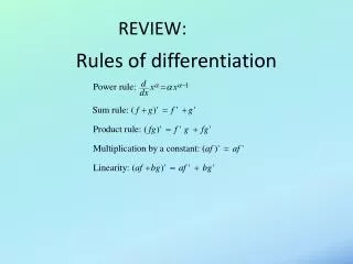
Rule 1: Derivative of a Constant • We will use the notation • To mean “the derivative off with respect tox at x.” Rule 1: Derivative of a constant • The derivative of a constant function is equal to zero.
Rule 1: Derivative of a Constant • We can see geometrically why the derivative of a constant must be zero. • The graph of a constant function is a straight line parallel to thexaxis. • Such a line has a slope that is constant with a value of zero. • Thus, the derivative of a constant must be zero as well. y f(x) = c x
Rule 1: Derivative of a Constant • We can use the definition of the derivative to demonstrate this:
Rule 2: The Power Rule Rule 2: The Power Rule • If n is any real number, then
Rule 2: The Power Rule • Lets verify this rule for the special case of n = 2. • If f(x) = x2, then
Rule 2: The Power Rule Practice Examples: • If f(x) = x, then • If f(x) = x8, then • If f(x) = x5/2, then Example 2, page 159
Rule 2: The Power Rule Practice Examples: • Find the derivative of Example 3, page 159
Rule 2: The Power Rule Practice Examples: • Find the derivative of Example 3, page 159
Rule 3: Derivative of a Constant Multiple Function Rule 3: Derivative of a Constant Multiple Function • If c is any constant real number, then
Rule 3: Derivative of a Constant Multiple Function Practice Examples: • Find the derivative of Example 4, page 160
Rule 3: Derivative of a Constant Multiple Function Practice Examples: • Find the derivative of Example 4, page 160
Rule 4: The Sum Rule Rule 4: The Sum Rule
Rule 4: The Sum Rule Practice Examples: • Find the derivative of Example 5, page 161
Rule 4: The Sum Rule Practice Examples: • Find the derivative of Example 5, page 161
Applied Example: Conservation of a Species • A group of marine biologists at the Neptune Institute of Oceanography recommended that a series of conservation measures be carried out over the next decade to save a certain species of whale from extinction. • After implementing the conservation measure, the population of this species is expected to be where N(t) denotes the population at the end of year t. • Find the rate of growth of the whale population when t= 2 and t= 6. • How large will the whale population be 8 years after implementing the conservation measures? Applied Example 7, page 162
Applied Example: Conservation of a Species Solution • The rate of growth of the whale population at any time t is given by • In particular, for t = 2, we have • And for t = 6, we have • Thus, the whale population’s rate of growth will be 34 whales per year after 2 years and 338 per year after 6 years. Applied Example 7, page 162
Applied Example: Conservation of a Species Solution • The whale population at the end of the eighth year will be Applied Example 7, page 162
3.2 The Product and Quotient Rules
Rule 5: The Product Rule • The derivative of the product of two differentiable functions is given by
Rule 5: The Product Rule Practice Examples: • Find the derivative of Example 1, page 172
Rule 5: The Product Rule Practice Examples: • Find the derivative of Example 2, page 172
Rule 6: The Quotient Rule • The derivative of the quotient of two differentiable functions is given by
Rule 6: The Quotient Rule Practice Examples: • Find the derivative of Example 3, page 173
Rule 6: The Quotient Rule Practice Examples: • Find the derivative of Example 4, page 173
Applied Example: Rate of Change of DVD Sales • The sales ( in millions of dollars) of DVDs of a hit movie t years from the date of release is given by • Find the rate at which the sales are changing at time t. • How fast are the sales changing at: • The time the DVDs are released (t = 0)? • And two years from the date of release (t = 2)? Applied Example 6, page 174
Applied Example: Rate of Change of DVD Sales Solution • The rate of change at which the sales are changing at time t is given by Applied Example 6, page 174
Applied Example: Rate of Change of DVD Sales Solution • The rate of change at which the sales are changing when the DVDs are released (t = 0) is That is, sales are increasing by $5 million per year. Applied Example 6, page 174
Applied Example: Rate of Change of DVD Sales Solution • The rate of changetwo years after the DVDs are released (t = 2) is That is, sales are decreasing by $600,000 per year. Applied Example 6, page 174
3.3 The Chain Rule
Deriving Composite Functions • Consider the function • To compute h′(x), we can first expandh(x) and then derive the resulting polynomial • But how should we derive a function like H(x)?
Deriving Composite Functions Note that is a composite function: • H(x) is composed of two simpler functions • So that • We can use this to find the derivative of H(x).
Deriving Composite Functions To find the derivative of the composite functionH(x): • We let u = f(x)= x2 + x + 1 and y = g(u) = u100. • Then we find the derivatives of each of these functions • The ratios of these derivatives suggest that • Substitutingx2 + x + 1 for u we get
Rule 7: The Chain Rule • If h(x)= g[f(x)], then • Equivalently, if we write y = h(x) = g(u), where u = f(x), then
The Chain Rule for Power Functions • Many composite functions have the special form h(x)= g[f(x)] where g is defined by the rule g(x) = xn(n,a real number) so that h(x)= [f(x)]n • In other words, the functionhis given by the power of a functionf. • Examples:
The General Power Rule • If the function f is differentiable and h(x)= [f(x)]n(n,a real number), then
The General Power Rule Practice Examples: • Find the derivative of Solution • Rewrite as a power function: • Apply the general power rule: Example 2, page 184
The General Power Rule Practice Examples: • Find the derivative of Solution • Apply the product rule and the general power rule: Example 3, page 185
The General Power Rule Practice Examples: • Find the derivative of Solution • Rewrite as a power function: • Apply the general power rule: Example 5, page 186
The General Power Rule Practice Examples: • Find the derivative of Solution • Apply the general power rule and the quotient rule: Example 6, page 186
Applied Problem: Arteriosclerosis • Arteriosclerosis begins during childhood when plaque forms in the arterial walls, blocking the flow of blood through the arteries and leading to heart attacks, stroke and gangrene. Applied Example 8, page 188
Applied Problem: Arteriosclerosis • Suppose the idealized cross section of the aorta is circular with radius acm and by year t the thickness of the plaque is h= g(t) cm then the area of the opening is given by A = p(a – h)2cm2 • Further suppose the radius of an individual’s artery is 1cm (a = 1) and the thickness of the plaque in year t is given by h = g(t) = 1 – 0.01(10,000 – t2)1/2 cm Applied Example 8, page 188
Applied Problem: Arteriosclerosis • Then we can use these functions for h and A h = g(t) = 1 – 0.01(10,000 – t2)1/2A = f(h) = p(1 – h)2 to find a function that gives us the rate at which A is changing with respect to time by applying the chain rule: Applied Example 8, page 188
Applied Problem: Arteriosclerosis • For example, at age 50 (t = 50), • So that • That is, the area of the arterial opening is decreasing at the rate of 0.03cm2 per year for a typical 50 year old. Applied Example 8, page 188
3.4 Marginal Functions in Economics
Marginal Analysis • Marginal analysis is the study of the rate of change of economic quantities. • These may have to do with the behavior of costs, revenues, profit, output, demand, etc. • In this section we will discuss the marginal analysis of various functions related to: • Cost • Average Cost • Revenue • Profit • Elasticity of Demand
Applied Example: Rate of Change of Cost Functions • Suppose the total cost in dollars incurred each week by Polaraire for manufacturing x refrigerators is given by the total cost function C(x) = 8000 + 200x – 0.2x2 (0 x 400) • What is the actual cost incurred for manufacturing the 251strefrigerator? • Find the rate of change of the total cost function with respect to x when x = 250. • Compare the results obtained in parts (a) and (b). Applied Example 1, page 194
Applied Example: Rate of Change of Cost Functions Solution • The cost incurred in producing the 251st refrigerator is C(251) – C(250) = [8000 + 200(251) – 0.2(251)2] – [8000 + 200(250) – 0.2(250)2] = 45,599.8 – 45,500 = 99.80 or $99.80. Applied Example 1, page 194