Download

1 / 13
130 likes | 208 Views
Population Based Optimization for Variable Operating Points. Alan L. Jennings & Ra úl Ordóñez, ajennings1 , raul.ordonez@notes.udayton.edu Electrical and Computer Engineering University of Dayton. Method. Examples. Introduction. Conclusion. Adjust X Many dimensions. The Challenge.

E N D
Population Based Optimization for Variable Operating Points Alan L. Jennings & Raúl Ordóñez, ajennings1, raul.ordonez@notes.udayton.edu Electrical and Computer Engineering University of Dayton Method Examples Introduction Conclusion CEC2011-#274
Adjust X Many dimensions The Challenge Change Y One dimension As a desired parameter changes, Smoothly change other parameters in real-time, While maintaining local optimality. The Solution Global search/optimization of input space, To form inverse functions in the output space, Using particles and clusters. Smoothly and quickly Maintain Optimality Method Examples Introduction Conclusion CEC2011-#274
Problem Statement • Find continuous functions x*= hi(yd) Such that, • J=g(x*) is local minimum • yd=f(x*) over an interval of yd. Assumptions • Compact set in x • g & f are C1, deterministic and time invariant • Change in x is easy to implement • Adequately scaled • Regions larger than a point where ∇f=0 can result in open domain of hi Method Examples Introduction Conclusion CEC2011-#274
Example Problems Input: Set point Output: Temperature Cost: Energy • Thermostat • Combining generators • Optimal control trajectory Linear, SISO system Input: Servo positions nodes in time This method is different from • Nominal operating point • Pareto-Optimal Front Output: Crawl distance, Jump height, …. Cost: Energy, Max Torque, Profile Height,… Method Examples Introduction Conclusion CEC2011-#274
Surrogate Function Creation Execution Swarm Optimization Method Overview Swarm Optimization Select cluster hi Sample Function Initialize Population • Neural Networks Universal Approximators Converge in the gradient Simple to get gradient • Swarm Optimization Agents cover n space Simple motions Allow for clusters • Spline Interpolation Use known optimal points of clusters Train Network Get yd Evaluate hi Move Agents: lower g(x), keep f(x) Move x to x* Validate Network Check for removal/ settling conditions Form clusters Execution Method Examples Introduction Conclusion CEC2011-#274
Particle Motion • Output gradient Move in null space • Cost gradient Move opposite (in null space) • Saturation All gradients saturate If gradients are large -> fixed step length If a gradient is small -> step size diminishes • Boundary constraint reduces step length • Minimum step for settling • Remove particles close to another Quickly reduces population size Output Cost Step Method Examples Introduction Conclusion CEC2011-#274
Cluster Formation • Form cluster from settled particle • Ascend/Descend Output Form new point Apply gradient descent • End Cluster conditions Particle doesn’t settle Output decreases / increases Settles too far away / close Method Examples Introduction Conclusion CEC2011-#274
Simple Example • Combination of generators Output: Total power out Cost: Quadratic function • Expected result Each does half the load Method Examples Introduction Conclusion CEC2011-#274
Complex Examples • Combination of functions Multiple extremum Saddle points 2-dim for verification • Expected result Clusters between output extremum Linear/Quadratic Cost Periodic Cost Quadratic Cost Quadratic Cost Method Examples Introduction Conclusion CEC2011-#274
Cluster 1 Test Cluster Evaluation • Verify Output Accuracy Plot Actual vs Desired for test points • Verify Optimality Generate neighbors Plot cost vs output Subtract expected cost Cluster 2 Test Method Examples Introduction Conclusion CEC2011-#274
5 Dim, ill scaled example • 5 different generators • Order of magnitude difference of gradient • Used exact NN to eliminate that source or error • Resulted in single cluster that balanced the incremental cost of all generators • 0.1% full range accuracy
Failure Methods • `Kill distance’ may end other bifurcation branches • Cluster ends prematurely • Global optimization parameters insufficient • Corners in clusters can impair cubic interpolation Piecewise cubic can make interpolant monotonic • Difficult to verify in high dimensions Testing cluster is reasonably simple Possible bifurcations, direction dependent Gradient goes to zero, ends cluster Corners in cluster interfere with interpolation Method Examples Introduction Conclusion CEC2011-#274
Questions or Comments? Global search, using particles & clusters, to find optimal, continuous output-inverse functions. _____________________________________________________________ Tested to work on many difficult combinations. _____________________________________________________________ Future: apply to developmental/ resolution increasing control Method Examples Introduction Conclusion CEC2011-#274