Download
1 / 37
370 likes | 578 Views
THE COMMUNITY MULTISCALE AIR QUALITY (CMAQ) MODEL: Model Configuration and Enhancements for 2006 Air Quality Forecasting. Rohit Mathur, Jonathan Pleim, Kenneth Schere, George Pouliot, Jeffrey Young, Tanya Otte Atmospheric Sciences Modeling Division ARL/NOAA NERL/U.S. EPA

E N D
THE COMMUNITY MULTISCALE AIR QUALITY (CMAQ) MODEL:Model Configuration and Enhancements for 2006 Air Quality Forecasting Rohit Mathur, Jonathan Pleim, Kenneth Schere, George Pouliot, Jeffrey Young, Tanya Otte Atmospheric Sciences Modeling Division ARL/NOAA NERL/U.S. EPA Hsin-Mu Lin, Daiwen Kang, Daniel Tong, Shaocai Yu, Science and Technology Corporation
Acknowledgements • Jeff McQueen, Pius Lee, Marina Tsidulko • Paula Davidson Disclaimer: The research presented here was performed under the Memorandum of Understanding between the U.S. Environmental Protection Agency (EPA) and the U.S. Department of Commerce’s National Oceanic and Atmospheric Administration (NOAA) and under agreement number DW13921548. This work constitutes a contribution to the NOAA Air Quality Program. Although it has been reviewed by EPA and NOAA and approved for publication, it does not necessarily reflect their views or policies.
Meteorological Observations WRF-NMM-CMAQ AQF System WRF-NMM NAM Meteorology model WRF Post Vertical interpolation Horizontal interpolation to Lambert grid PRDGEN PREMAQ CMAQ-ready meteorology and emissions CMAQ Emission Inventory Data Chemistry/Transport/Deposition model AQF Post Gridded ozone files for users Verification Tools Performance feedback for users/developers Air Quality Observations
CMAQ Modeling Domains Experimental PM forecasts on 5x Ozone forecasts both domains 12 km resolution 265 grid cells 259 grid cells CONUS “5x” Domain Experimental East “3x” Domain 268 grid cells 442 grid cells
Emission Processing • Emission Processing is a component of PREMAQ (pre-processor to CMAQ) • Point Source and Biogenic Source processing from SMOKE • Area Sources (no meteorological modulation) computed in SMOKE outside of PREMAQ • Mobile Sources (nonlinear least squares approximation to SMOKE/Mobile6)
Area and Biogenic Sources • Area Sources: Computed outside of PREMAQ • 2001 NEI version 3 inventory used. (CAIR) No changes made to inventory. • Replaced year specific with average (1996-2002) estimates for fires • Biogenic Sources: BEIS3.13 included directly into PREMAQ. • Canadian Inventory: 1995 used (includes all provinces) • Mexican Inventory: BRAVO 1999 used for point sources
Mobile Sources • SMOKE/MOBILE6 not efficient for real-time forecasting • SMOKE/MOBILE6 used to create retrospective emissions for AQF grid • 2006 (projected from 2001) VMT data used for input to Mobile 6 • 2006 Vehicle Fleet used for input to Mobile 6 • For 13 counties in Metropolitan Atlanta area, VMT based on 2005 run of a travel demand model and Mobile6 inputs from Georgia DNR
Mobile Sources • Regression applied at each grid cell at each hour of the week for each species to create temperature/emission relationship • Mobile Source emissions calculated in real-time using this derived temperature/emission relationship • For California used 2001 mobile estimates from • CARB
NE Domain Mobile6 vs. Regression: NOx Saturday Monday
NE Domain Mobile6 vs. Regression: VOC Saturday Monday
Point Sources • 2004 Continuous Emissions Monitoring for NOx and SO2 • Monthly temporal profiles on a state-by-state basis derived from 2004 CEM • For other pollutants and non-EGU: 2001 NEIv3 • Georgia non-EGU based on 2002 inventory from GADNR • Modified EGU NOx emissions using DOE’s Annual Energy Outlook (Jan. 2006) • Calculated 2006/2004 NOx and SO2 annual emission ratios on a regional basis (from DOE data) • Exception California
EGU NOX adjustments 2006/2004 by region 1.20 1.56 1.64 1.12 1.11 0.98 1.01 1.0 1.02 0.95 0.84 DOE/AOE estimated an increase by factor of 8 1.03 0.74 Source: Department of Energy Annual Energy Outlook 2006 http://www.eia.doe.gov/oiaf/aeo/index.html
CMAQ Configuration • Advection • Horizontal: Piecewise Parabolic Method • Vertical: Upstream with rediagnosed vertical velocity to satisfy mass conservation • Turbulent Mixing • K-theory; PBL height from WRF-NMM • Minimum value of Kz allowed to vary spatially depending on urban fraction (furban) • Kz = 0.1 m2/s, furban = 0 • Kz = 2.0 m2/s, furban = 1 • allows min. Kz in rural areas to fall off to lower values than urban regions during night-time • prevents precursor concentrations (e.g., CO, NOx) in urban areas from becoming too large at night; reduced mixing intensity) in non-urban areas results in increased night-time O3 titration
CMAQ Configuration (contd.) • Gas phase chemistry • CB4 mechanism with EBI solver • Below cloud attenuation based on ratio of radiation reaching the surface to its clear-sky value • Closer linkage with the NAM fields • Cloud Processes • Mixing and aqueous chemistry • Scavenging and wet deposition • Sub-grid scheme based on modifications to RADM formulation; “switch-off” entrainment from above clouds • Used in Eastern U.S. (3x) domain • “In-cloud” mixing based on the Asymmetric Convective Mixing (ACM) model (Pleim and Chang, 1992, JGR) • Used in Continental U.S. (5x) domain
CMAQ Configuration (contd.) O3 Deposition Velocity Stomatal Conductance • Deposition • Dry : M3dry modified to use WRF land surface parameters • Changes in WRF-LSM impact Vdo3 (relative to Eta) • Persistent sink for O3 – can impact predicted O3 ETA ETA WRF WRF
HNO3 EC NO3- NH4+ SO4= Na+ Cl- H2O NH3 POA SOAa SOAb H2SO4 Aromatics Other Monoterpenes HCl H2O • Trimodal size distribution • Aitken (0-0.1 µm), Accumulation(0.1-2.5 µm), • and Coarse • Gas/particle interactions treated for fine modes only – ISORROPIA instantaneous equilibrium • Fine-modes coagulate • Coarse mode, fine EC (black) & other fine PM (brown) are inert CMAQ Configuration: Aerosols Binkowski and Roselle, JGR, 2002 SVOCs Na+, Cl-, SO42- Soil, Other 2 FINE MODES COARSE MODE
Structural Enhancements • Included layer dependent advection time-step calculation • Improves model efficiency • Coupling between WRF-NMM and CMAQ • “Loose-coupling” (used in Operational 3X) • Similar to previous Eta-CMAQ linkage • WRF-NMM and CMAQ coordinate and grid structures are different. Interpolation of meteorological inputs to the CMAQ grid and coordinate • “Tight-coupling” (implemented in Experimental 5X) • Step 1: Coupling in the vertical implemented this summer • CMAQ calculations on the same vertical coordinate as WRF-NMM • Step 2: Modifications to CMAQ to facilitate calculations on native WRF-NMM horizontal grid • Stay tuned
PT PDT PD Ps = PD + PDT + PT WRF-NMM Hybrid Vertical Coordinate System“Tightly Coupled”
Tightly Coupled System Conversion to use WRF-NMM vertical coordinate in PREMAQ and CMAQ s’s limited to 0-1 Jacobian: encapsulates coordinate transformations between physical and computational space Jacobian across the interface
Comparison of Experimental and Operational Forecasts Mean over sites within Operational 3x Domain 5X under-predictions at peak values
Comparison of Experimental and Operational Forecasts Operational (3X) Developmental (5X) 5X vs. 3X: Regionally lower O3; under-prediction of peak values
Diagnosing the low-bias in Experimental 5X Runs California Sub-domain average time series: July 18-19, 2006 Black (Loose), Red (Tight w/ISOP error), Green (Corrected Tight) NTR: Inert organic nitrate in CBM-IV NTR Isoprene Ozone
Correcting the low-bias in Experimental 5X Runs Max.-8hr O3: 7/19/06 IsopreneFix Tight Old Tight Loose
Correcting the low-bias in Experimental 5X Runs Loose Max. 8 O3 7/19/06 Old Tight Isoprene Fix Tight
Improvements from Tight Coupling Mass-consistent advection Vertical Velocity Cross-sections Tight coupling helps reproduce WRF-NMM vertical velocity fields with higher fidelity Note: Large discrepancies at model top in loose-coupling
Lateral Boundary Condition Specification • A key uncertainty in long term modeling over limited area domains • Determines “model background” • Approach in Operational Runs: Combination of • Static default profiles • “Clean” tropospheric background values • Top most CMAQ-layer: O3 profiles from NCEP’s Global Forecast System (GFS) model • O3 is a 3-d prognostic variable • Initialized with Solar Backscatter Ultra-Violet (SBUV-2) satellite observations • Approach in Experimental Runs • Static default profiles • Added diagnostic tracers to quantify “model background” O3 • Tracked impact of lateral boundary conditions (surface-3km and 3km-model top)
Modeled surface-level “background” O3 Average from July 1-August 22, 2006 Background O3 distributions are spatially heterogeneous
Components of modeled surface-level “background” O3 “Boundary Layer” Surface – 3km “Free Troposphere” 3km – Model top
Components Modeled “background” O3: Relative Contributions/Fraction “Boundary Layer” Surface – 3km “Free Troposphere” 3km – Model top
Performance Summary for PM2.5 over a year: 2005 Captures day-to- day variability Warm-season Under-prediction Cool-season Over-prediction
Performance Summary over a year: 2005 Larger errors at higher concentrations • Winter high bias • Possible measurement bias • Role of dynamics • Unspeciated “Other” PM is biased high
2/2/05 2/1/05 2/3/05 2/4/05 2/5/05 2/6/05 Model Performance Characteristics: Winter 2005 Model and Observed Daily Average Surface PM2.5 μg/m3 5 10 15 20 25 30 35 • Capture hot-spots, tendency to over-predict • possible role of mixing; Kzmin and/or PBL height ?
PM2.5 Compositional Characteristics STN Measurements Winter 2005 Summer 2004 • Reasonable representation of Inorganic • compositional characteristics • Sulfate fraction over-predicted • Organic fraction under-predicted • Nitrate is a bigger player • Larger OC fraction • under-predictions at lower • concentrations
Specification of “Real Time” Emissions Testing HMS-HYSPLIT fire emissions algorithm Without Fires With Fires Difference June 24, 2005: Daily Avg. PM2.5 Cave Creek Complex fire began as two lightning-sparked fires on June 21, 2005. Became second largest fire in Arizona history.
Specification of “Real Time” Emissions Testing HMS-HYSPLIT fire emissions algorithm June 21-26, 2005 Daily Avg.: Southern NV sites Fire plume signatures: June 24, 2005 Real-time specification of fire emissions improves PM forecast skill June 24, 2005
Summary/Looking Ahead • AQF system transitioned to WRF-NMM • Growing pains with a new and evolving modeling system • WRF-NMM based dry-deposition velocities are higher than those derived from Eta • Persistent sink- can systematically impact predicted O3 • Implemented the first step in tighter coupling between CMAQ and WRF-NMM computational grids • CMAQ calculations using the WRF-NMM vertical coordinate • Modifications to CMAQ to use the E-grid and rotated lat/lon coordinate underway • Under-predictions for surface O3 in experimental predictions were found to arise from error in isoprene emission calculations • Un-initialized lat/lon fields
Summary/Looking Ahead • Initial analysis of boundary tracers indicate that modeled O3 background values are strongly influenced by free tropospheric LBC values • Locations at which O3 is over-predicted generally also correspond to high background but low observed values • Rigorous analysis of developmental PM simulations underway • Seasonal trends/biases similar to hind-cast CMAQ applications • Speciated PM verifications with surface network (STN, CASTNet, IMPROVE, SEARCH) and aloft (ICARTT) data • Initial testing of a methodology for specifying “real-time” fire emissions tested • Initial results are encouraging