Download
1 / 9
90 likes | 200 Views
Learn about building a virtual camera to transform 4D light fields into 2D images using optical elements and software simulation. Explore challenges and motivations in computational camera research.

E N D
Virtual Computational Camera Changyin Zhou changyin@cs.columbia.edu Computational Photography, Spring 2009
2D Sensor Lens, Lens Array,Coded Aperture, 3D Phase plate …. Illumination 4D Light Field - Camera is a projection: [4D light field] [2D image] Shape, BRDF Input: Transforms … Input: 4D light field Ouput: 2D image What is Camera? - Optical Elements are transforms: [4D Light Field] [4D Light Field]
Optical Simulation Software (Zemax, ASAP…) From Scratch (using Matlab, Python, C, …) Works as a real system in most cases - Ray tracing - Optical Element Based • Define Optical Elements Physically • (e.g. curvatures of surface, refractive index) - Not well structured for optical design • Not easy to develop from scratch • (little intuition, time-consuming, …) Disadvantage: • No light field … • A big gap between physics and math • Designed for conventional optical elements • Coded aperture? • Focal Sweep? Motivation Two Typical Ways to Build Virtual Cameras
Input: Transforms… Input: 4D light field Output: 2D image Build An Abstract-Level Virtual Camera Purpose: Serve Computational Camera Research Sensor: Projection: 4D Light Field 2D Image An Abstract-Level Virtual Camera Scene: 4D Light Field Features: 1. Light Field Based 2. “Object-Oriented”: Optical Elements Optical Element: Transform of 4D Light Field 3. Concept-Level: Defined mathematically 4. Pipeline
Build An Abstract-Level Virtual Camera • Sensor: • function outIM = sensor(inLF, inDist); • For each [u, v] • outIM(round(XX(1, :)*desU), round(YY(:, 1)'*desV) … • = outIM(round(XX(1, :)*desU), round(YY(:, 1)'*desV)… • + interp2(XX, YY, inLF{u, v}, … • round(XX*desU)/desU, round(YY*desV)/desV); • end Scene: LF(u, v, s, t) Lens: function outLF = Lens(inLF, arg); For each [u, v] outLF{u, v} = interp2(X, Y, inLF{u, v}, X-u/f, Y-v/f); end Any other element: function outLF = Other(inLF, arg); …. …. ….
Build An Abstract-Level Virtual Camera Camera Function VirtualCamera(parameters); LF = loadLF(filename); LF = lens(LF, arg); LF = codedAperture(LF, coding, arg); LF = propagation(LF, distance); LF = otherOptics(LF, arg); LF = propagation(LF, distance); IM = sensor(LF); END
Challenges • Resolution • Huge data (Constrained to 10 x 10 x 1000 x 1000 input light field in this project) • Angular/spatial resolution balance could be different at every layer. • An effective Framework (user interface, data structure, function interface, …) • Ray Interpolation