Download
1 / 10
100 likes | 217 Views
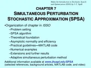
Slides for Introduction to Stochastic Search and Optimization ( ISSO ) by J. C. Spall. CHAPTER 5 S TOCHASTIC G RADIENT F ORM OF S TOCHASTIC A PROXIMATION. Organization of chapter in ISSO Stochastic gradient Core algorithm Basic principles Nonlinear regression Connections to LMS

E N D
Slides for Introduction to Stochastic Search and Optimization (ISSO)by J. C. Spall CHAPTER 5STOCHASTIC GRADIENT FORM OF STOCHASTIC APROXIMATION Organization of chapter in ISSO Stochastic gradient Core algorithm Basic principles Nonlinear regression Connections to LMS Neural network training Discrete event dynamic systems Image processing
Stochastic Gradient Formulation • For differentiable L(), recall familiar set of p equations and p unknowns for use in finding a minimum : • Above is special case of root-finding problem • Suppose cannot observe L() and g() except in presence of noise • Adaptive control (target tracking) • Simulation-based optimization • Etc. • Seek unbiased measurementof L/ for optimization
Stochastic Gradient Formulation (Cont’d) • Suppose L() = E[Q(,V)] • Vrepresents all random effects • Q(,V) represents “observed” cost (noisy measurement of L()) • Seek a representation where Q/is an unbiased measurement ofL/ • Not true when distribution function for V depends on • Above implies that desiredrepresentation is not where pV() is density function for V
Stochastic Gradient Measurement and Algorithm • When density pV() is independent of , is unbiased measurement of L/ • Above requires derivative–integral interchange in L/ =E[Q(,V)]/ = E[Q(,V)/] to be valid • Can use root-finding (Robbins-Monro) SA algorithm to attempt to find : • Unbiased measurement satisfies key convergence conditions of SA (Section 4.3 in ISSO)
Stochastic Gradient Tendency to Move Iterate in Correct Direction
Stochastic Gradient and LMS Connections • Recall basic linear model from Chapter 3: • Consider standard MSE loss: L()= • Implies Q = • Recall basic LMS algorithm from Chapter 3 • Hence LMS is direct application of stochastic gradient SA • Proposition 5.1 in ISSO shows how SA convergence theory applies to LMS • Implies convergence of LMS to
Neural Networks • Neural networks (NNs) are general function approximators • Actual output zk represented by a NN according to standard model zk= h(,xk) + vk • h(,xk) represents NN output for input xk and weight values • vkrepresents noise • Diagram of simple feedforward NN on next slide • Most popular training method is backpropagation (mean-squared-type loss function) • Backpropagation is following stochastic gradient recursion
Simple Feedforward Neural Network with p = 25 Weight Parameters
Discrete-Event Dynamic Systems • Many applications of stochastic gradient methods in simulation-based optimization • Discrete-event dynamic systems frequently modeled by simulation • Trajectories of process are piecewise constant • Derivative–integral interchange critical • Interchange not valid in many realistic systems • Interchange condition checked on case-by-case basis • Overall approach requires knowledge of inner workings of simulation • Needed to obtain Q(,V)/ • Chapters 14 and 15 of ISSO have extensive discussion of simulation-based optimization
Image Restoration • Aim is to recover true image subject to having recorded image corrupted by noise • Common to construct least-squares type problem where Hs represents a convolution of the measurement process (H) and the true pixel-by-pixel image (s) • Can be solved by either batch linear regression methods or the LMS/RLS methods • Nonlinear measurements need full power of stochastic gradient method • Measurements modeled as Z = F(s,x,V)